Residuals are the errors in the predictions of your linear model for each observation. Because yours is a simple linear model, your errors look a lot like your observations, but they are not exactly identical. Your regression line in the first scatterplot is essentially the same as the horizontal dotted line in your second scatterplot, "Residuals vs. Fitted"Residuals vs. Fitted, but angled upward to reflect a positive correlation between year and rainfall, and passing through different coordinates. Hence the pattern only differs between these two scatterplots in terms of that angular rotation and the locations of your coordinates. I.e., your "Residuals vs. Fitted"Residuals vs. Fitted scatterplot rotated and relocated the data coordinates so that your scatterplot axes $x_1$$x$ and $y_1$$y$ axes changed from YearYear and Rainfall valuesRainfall, respectively, to:
$$x_2=\text{intercept coefficient}+\text{slope coefficient}\cdot x_1$$$$x_{\text{Residuals vs. Fitted}}= \text{Year}\times\text{slope}+\text{intercept }\\\ \
y_{\text{Residuals vs. Fitted}}=\text{Rainfall} - x_{\text{Residuals vs. Fitted}}$$
$$y_2=y_1 - x_2$$
@charles' answerThus your slope coefficient determines the change in angle and your intercept coefficient changes the location of the observation pattern in your coordinate space. If either were closer to zero, your patterns would be that much more identical. Either value being exactly zero is a good responseperfectly tolerable and potentially meaningful result for a linear regression. In fact, these represent the null hypotheses of typical $t$ tests for those coefficients, so they have to whether you should've usedbe tolerable and interpretable results – otherwise, one could not really try to falsify those nulls this particular modelway (however, andregression is not a NHST inherently).
@Penguin_Knight's answer is a useful alternative phrasing of my point here, with an additional consideration of multiple regression, which you may want to consider if you have other independent variables you'd like to relate to rainfall. I hope I wasn't@charles' answer is an interesting response to whether you should've used this particular model. Building on that, here are some other points to consider:
Your
Residuals vs. Fittedplot has a convex, locally weighted scatterplot smoothing (loess) line drawn through it, if I'm not mistaken. Because it's convex, you might want to try polynomial regression or other curve-fitting approaches if you can get more data...but with 21 observations only (one per year, right?), these are exercises in overfitting. Their utility depends on your purpose.I tried eyeballing your
Rainfalldata as roughly the following:Rainfall=c(45,36,53,52,52,43,41,47,55,54,68,47,63,42,57,50,61,60,65,55,47)
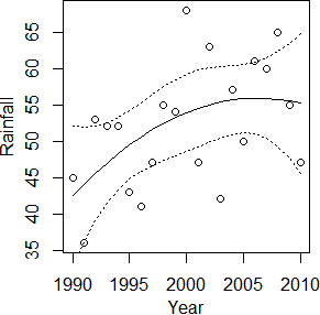
then triedsummary(lm(Rainfall~Year+Year2))whereYear=1990:2010andYear2=scale(Year,scale=F)^2(Can't seem to squareYearinsidelm()...). Here's what I got: $$\text{Rainfall}=.64\times\text{Year}-.05\times\text{Year}^2-122$$ This worsened the model's $F$ and $R^2$, and with $t_{(18)}=-.99,p=.34$ for the quadratic term, I wouldn't reject a null hypothesis that denies a curvilinear relationship, but it is prettier: produced with
 curveplot(Year,Rainfall)where
curveplot=function(x,y){plot(x,y);x2=scale(x,scale=F)^2; lines(x,predict(lm(y~x+x2))) lines(x,predict(lm(y~x+x2),interval='confidence')[,2],lty=3) #(these two lines plot lines(x,predict(lm(y~x+x2),interval='confidence')[,3],lty=3)} #(95% confidence-intervals)
You may want to run this function on your actual data, since my eyeballs distorted yourRainfalldata...or you might not. It's a more complex model, it might be overfitted, and there's really not enough evidence of a curvilinear trend. If you were modeling a longer period of time or trying to predict rainfall for years outside 1990–2010, it's almost certain that you wouldn't want a quadraticYearterm, because it causes the $\lim_{\text{Year}\rightarrow\pm\infty}=-\infty$ (so long as it's negative, as here). Hence I only suggest it in case you want to describe the gradually decreasing slope in this specific time frame with a relatively simplistic model (e.g., as evidence against a strong curve). Also, I wanted to show off a simple confidence interval plot!If you have more precise information about the times of your observations – e.g., if they weren't exactly annual, and you know how many days/weeks/months short of a full year each observation of
Rainfallpertains to – you might want to improve the precision of yourYearvalues, because a simple linear regression model fit with OLS assumes your variables are continuous. E.g., if 1995's observation pertains to the sum of rainfall measurements beginning after the last rainfall measurement of 1994 on December 25 and ending with the last rainfall of 1995 on December 6, you might consider setting the value ofYearcorresponding to that sixth observation ofRainfallto be $\frac{346}{365}$ higher than the previous value, not exactly 1 higher. You might not want to either; it complicates your work, and it shouldn't matter much as long as the real time differences between your observations don't vary too much.
Annual rainfall measurements between 35–70mm implies incredible aridity though – even Antarctica gets more precipitation than that, mostly. Even if you actually meant centimeters, this is probably still a desert. If it's not raining often in your region of interest, your real time differences between observations might vary widely. If you can preserve that information, you should. Also, if you have info on separate observations within years that you are summing to simplify your analysis, bear in mind that this is reducing the accuracy of your model too slow. Annual rainfall accumulates as a nonlinear function of day-of-year, and in respondingarid climates, zero-inflation may be useful to incorporate in the model, because many days won't see any rain.
If you can model Rainfall over time with disaggregated measurements and specific dates, you'll also have to worry more about seasonal cycles after all, following charles' original reasoning. Never fear though; we'll be ofhappy to help as well!you pick the right model for that kind of data too, if you describe its disaggregated nature in a separate question (i.e., I wouldn't try to change this question to describe it). If your data is necessarily aggregated to the annual level, and if you don't have specific measurement dates, you can disregard most of this point, unfortunately.
- Another problem with OLS regression for these data may be implied by your
Normal Q-Qplot. OLS regression also assumes normally distributed residuals. It looks like yours have excess kurtosis, though maybe not too much. Regardless, you might consider robust or nonparametric alternatives to OLS linear regression. Some sacrifice power, but you might prefer to play it safe.
