1
$\begingroup$

It is commonly stated that "balanced" designs in multifactor ANOVA (equal sample sizes in each group) have "orthogonal" factors. In other regression contexts, I totally get the connection between the geometry (things at right angles to each other) and the statistics. Like how a residual vector is orthogonal to a least-squares solution because the latter is the projection of the response variable vector onto the column space of the design matrix. That makes perfect sense to me.

But for ANOVA, I'm at a loss. I can't figure out how factors in ANOVA correspond to some kind of geometric objects that are orthogonal. Even more perplexing is how this can only depend on the sample size in each group.

What am I missing? Can someone explain what geometric objects are supposed to correspond to "orthogonal" factors and why their orthogonality is a function only of the sample size in each group?

$\endgroup$
4
  • $\begingroup$ It is the columns of the design matrix in ANOVA that are orthogonal in the cell means model formulation. This treats the multifactor ANOVA as a one-way ANOVA with many classes $\endgroup$
    – user277126
    Commented Dec 1, 2021 at 4:43
  • $\begingroup$ I've written down the design matrix and (1) the columns do not appear to be orthogonal, and (2) even if they were, I fail to see how equal sample sizes would contribute to that. $\endgroup$ Commented Dec 1, 2021 at 19:49
  • $\begingroup$ Your original claim is baseless that "balanced designs" have anything to do with orthogonality. Also, you must have not expressed the ANOVA model as a cell means model, or else you'd see its columns are orthogonal, even for an unbalanced design. $\endgroup$
    – user277126
    Commented Dec 6, 2021 at 13:20
  • $\begingroup$ @user277126, rather than just a drive-by comment calling my question "baseless", it would be more helpful to post an answer showing the design matrix of the cell means model as an answer so I can see where I may have gone wrong. Also, for the record, the sum of squares for many, many ANOVA calculations I've done over the years show that the claim is not baseless. For example, Type I ANOVA only yields the same answers independent of entering the factors into the model (neatly partitioning the SS) when the sample sizes are equal across groups. $\endgroup$ Commented Dec 7, 2021 at 14:35

2 Answers 2

1
$\begingroup$

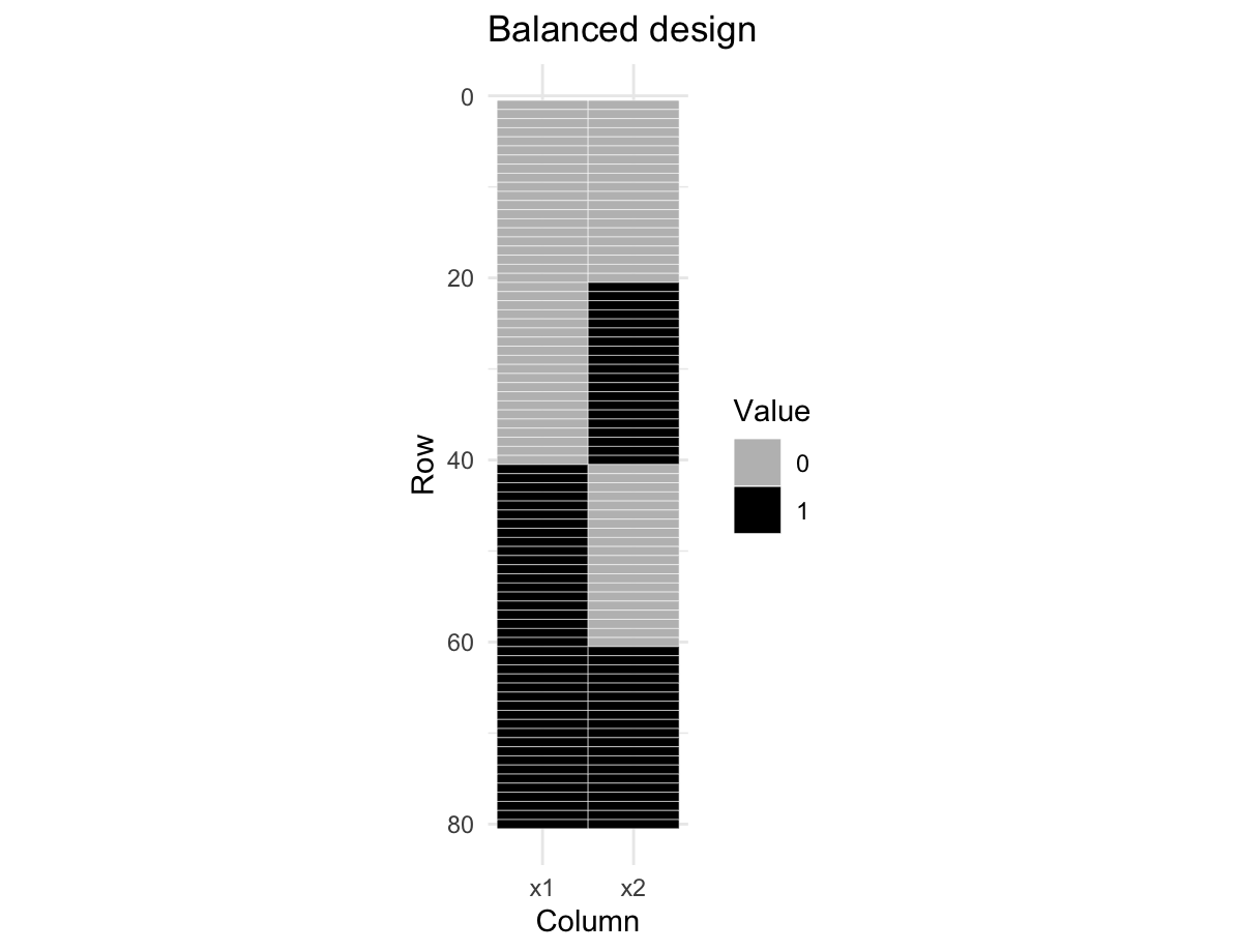
Let's take a simple 2x2 ANOVA, with two factors, x1 and x2, each of which can take one of two values, 0 and 1. There are therefore four cells in the design: [x1=0,x2=0], [0,1], [1,0], and [1,1].

In a balanced design, there are equal numbers of cases in each cell.

enter image description here

As a result, the two factors, x1 and x2 are uncorrelated (orthogonal), $r = 0$.

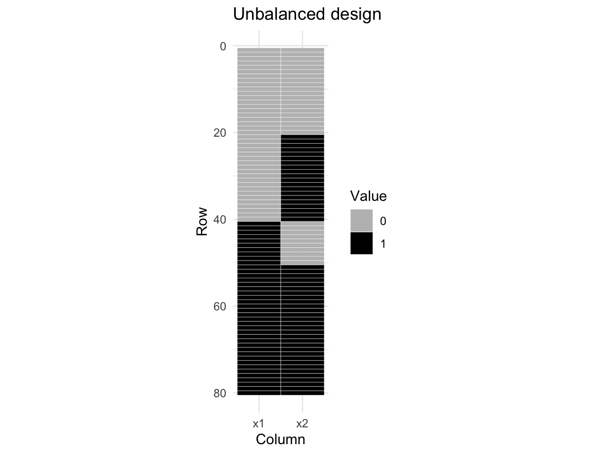
In an unbalanced design, there are more cases in some cells than others.

enter image description here

As a result, the factors are not uncorrelated, and so not orthogonal: in this example, cases where x1=1 are more likely to have x2=1, $r \approx .25$.

Demo code

library(tidyverse)
plot_design = function(df){
  long = df %>% 
    mutate(.index=1:n()) %>%
    pivot_longer(-.index)
  ggplot(long, aes(name, -.index, fill = factor(value))) +
    geom_tile(color = 'white') +
    scale_fill_manual(values = c('grey', 'black')) +
    labs(x = 'Column', y = 'Row', fill = 'Value') +
    scale_y_continuous(labels = function(x) -x) +
    theme_minimal() + coord_fixed(ratio = .1)
}

balanced_ns = c(20, 20, 20, 20)
df_balanced = data.frame(
  x1 = rep(c(0, 0, 1,1), times = balanced_ns),
  x2 = rep(c(0, 1, 0, 1), times = balanced_ns)
)
plot_design(df_balanced) + labs(title = 'Balanced design') # First figure, above
cor(df_balanced)
##    x1 x2
## x1  1  0
## x2  0  1


unbalanced_ns = c(20, 20, 10, 30)
df_unbalanced = data.frame(
  x1 = rep(c(0, 0, 1, 1), times = unbalanced_ns),
  x2 = rep(c(0, 1, 0, 1), times = unbalanced_ns)
)
plot_design(df_unbalanced) + labs(title = 'Unbalanced design') # Second figure
cor(df_unbalanced)
##           x1        x2
## x1 1.0000000 0.2581989
## x2 0.2581989 1.0000000
```
$\endgroup$
2
  • $\begingroup$ This is getting much closer to the answer I was looking for. I will note that the vectors that represent the two balanced factors in the design matrix are not orthogonal. (Their inner product will be 20--the number of cases where both take value 1.) But the fact that they are uncorrelated means some transformation of those vectors will be orthogonal. So I think this is pretty close. $\endgroup$ Commented Dec 10, 2021 at 18:31
  • $\begingroup$ Yes, I was a bit sloppy in my wording - if you want actual orthogonality, not just independence, code the values as -1 and +1. If this answers your question, please remember to upvote and mark the question as answered. $\endgroup$
    – Eoin
    Commented Dec 11, 2021 at 20:21
0
$\begingroup$

I'll take a stab at this one, but first from a non-geometric perspective. In probability, we estimate the joint probability of two random events using the following equation:

$p(A\cap B) = p(A)\times p(B)$

We can use this equation to also calculate the deviations from independence:

$\text{observed} - \text{expected under independence} = P(A\cap B) - P(A)\times P(B)$

where $P$ represents the observed probability. (Sorry if my notation is terrible...it's not my forte).

This is exactly what the traditional chi-square test of independence uses, but it replaces probabilities with counts:

expected = row sum $\times$ col sums / table sum

So, with an ANOVA, if your sample sizes are equal in each cell, they will be independent (orthogonal) because row sums $\times$ colsums / table sums will always exactly equal the expected probability as with a chi-square test.

Or, a different way to think about it is this: assuming a random process, it would be highly unusual to have a sample where the number of males/females over 6 feet tall are equal. Why would that be unusual? Because height is NOT independent of gender.

Likewise, for an ANOVA, if we have uncorrelated variables, they should have equal sample sizes. If they're correlated, they should not.

Make sense?

Geometric Explanation

This may be better to "see" than to explain. Let's say we have two factors (a and b) where the sample sizes are the same. The R code below generates the data and plots it. If we plot a against b (or vice versa), the best fitted regression line is exactly flat:

a = c(rep(c(1,2), times=6))
b = c(rep(1, times=6), rep(2, times=6))
d = data.frame(a=a,b=b)
table(a,b) #verify orthogonality
require(ggplot2)
ggplot(data=d, aes(x=a, y=b)) +
  geom_jitter(width=.1, height = .1) +
  geom_smooth(method="lm") # flat line
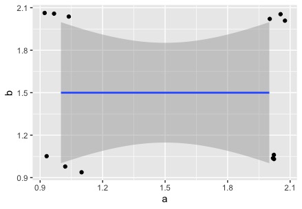
enter image description here

If we now allow different sample sizes in each group, there's now a positive slope:

a = c(rep(c(1,2), times=6))
b = c(rep(1, times=3), rep(2, times=9))
d = data.frame(a=a,b=b)
table(a,b) #verify nonorthogonality
ggplot(data=d, aes(x=a, y=b)) +
  geom_jitter(width=.1, height = .1) +
  geom_smooth(method="lm") # nonflat line
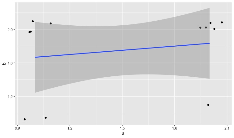
enter image description here

$\endgroup$
4
  • $\begingroup$ I'm not sure I completely buy either explanation. In the first half, I honestly don't see the connection you're trying to make with chi-square. There are no row sums, column sums, or table sums in ANOVA (unless I'm misunderstanding your point). And the second explanation isn't clear either. What does the regression line here have to do with ANOVA? Either way, I'm still looking for orthogonality of some vectors somewhere. $\endgroup$ Commented Dec 6, 2021 at 6:07
  • $\begingroup$ The deviations from independence defined above is similar to what I call the independence gap, although the joint need not be 'observed' necessarily in the case of the independence gap. Estimates can be substituted mutatis mutandis. $\endgroup$
    – Galen
    Commented Aug 4, 2023 at 3:35
  • $\begingroup$ "[...] with an ANOVA [...] they will be independent (orthogonal)" Yeah, for a (standard) ANOVA that holds since the covariance matrix fully specifies statistical dependence for a normal distribution. More generally statistical independence and orthogonality of random variables are not the same thing. $\endgroup$
    – Galen
    Commented Aug 4, 2023 at 3:41
  • $\begingroup$ "for an ANOVA, if we have uncorrelated variables, they should have equal sample sizes. If they're correlated, they should not." On the face of it this doesn't seem true. Can you elaborate and clarify? $\endgroup$
    – Galen
    Commented Aug 4, 2023 at 3:44

Your Answer

By clicking “Post Your Answer”, you agree to our terms of service and acknowledge you have read our privacy policy.

Not the answer you're looking for? Browse other questions tagged or ask your own question.