A simple approach would be to bootstrap means.
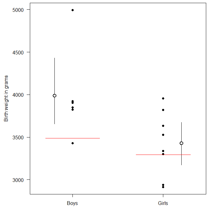
For the boys, this yields $p<0.0001$, that is, out of my 10,000 bootstrapped means, not a single one was below the boys' population mean weight.
For the girls, I get $p=0.15$ for the comparison of the bootstrapped mean against the population mean (i.e., 15% of my bootstrapped means are below the population mean).
In principle, you should really adjust these p-values for the multiple (two) tests you ran... but that won't make a difference, since $p=0$ will remain zero for the boys, and the nonsignificant result for the girls will remain nonsignificant.
Below is a plot of all your data, with group means and bootstrapped 95% confidence intervals for the means, and the population mean in red. If you had more data, you should really jitter the points horizontally.

Needless to say (I hope), you should be really careful about drawing conclusions from data samples this small.
R code:
boys <- c(3850, 4995, 3925, 3430, 3825, 3905)
girls <- c(3955, 3635, 3530, 2940, 3820, 3300, 2915, 3340)
population_boys <- 3487
population_girls <- 3293

library(boot)

# Boys:
set.seed(1) # for reproducibility
boot_boys <- boot(boys,function(x,i)mean(x[i]),R=10000)
boot_boys$t0	# mean
sd(boot_boys$t)   # standard error of the bootstrapped mean
ecdf(boot_boys$t)(population_boys)  # p value for one-sided test for equality with the population average

# Girls:
set.seed(1) # for reproducibility
boot_girls <- boot(girls,function(x,i)mean(x[i]),R=10000)
boot_girls$t0	# mean
sd(boot_girls$t)  # standard error of the bootstrapped mean
ecdf(boot_girls$t)(population_girls)    # p value for one-sided test for equality with the population average

opar <- par(mai=c(.5,1,.1,.1))
    plot(c(.6,2.4),range(c(boys,girls,population_boys,population_girls)),
        type="n",xlab="",ylab="",las=1,xaxt="n")
    mtext("Birth weight in grams",2,line=3.5)
    axis(1,c(1,2),c("Boys","Girls"))
    # plot boys
    points(rep(1,length(boys)),boys,pch=19)
    lines(c(0.8,0.8),quantile(boot_boys$t,c(0.025,0.975)))
	points(0.8,boot_boys$t0,pch=21,bg="white",cex=1.5,lwd=2)
    # plot girls
    points(rep(2,length(girls)),girls,pch=19)
    lines(c(2.2,2.2),quantile(boot_girls$t,c(0.025,0.975)))
	points(2.2,boot_girls$t0,pch=21,bg="white",cex=1.5,lwd=2)
    # plot population
    lines(c(.7,1.3),rep(population_boys,2),col="red")
    lines(c(1.7,2.3),rep(population_girls,2),col="red")
par(opar)


