A fundamental result in order statistics is Theorem 2.4.2 of Balakrishnan & Cohen:
Let $X_1, X_2, \ldots, X_n$ be i.i.id. random variables from a population with cdf $F$ and pdf $f,$ and let $X_{1:n}\le X_{2:n} \le \ldots \le X_{n:n}$ be the corresponding order statistics. Then the conditional distribution of $X_{i:n},$ given $X_{j:n}=x_{j;n},$ is the same as the distribution of the ith order statistic in a sample of size $j-1$ from a population with distribution $F$ truncated on the right at $x_{j:n}.$
It is straightforward to demonstrate and intuitive enough to be memorable. It says that when you know the $j^\text{th}$ largest value in a random sample from a known (continuous) distribution is $x_{j:n},$ the $j-1$ smaller values are distributed like a sample from all members of the population smaller than $x_{j:n}.$
Observe that $X_1=X_{n:n}$ (the maximum) with probability $1/n$ and otherwise $X_1$ is equally likely to be any of the $X_{(j)}$ for $1\le j \lt n.$ Applying the theorem to the case $j=n$ tells us the distribution of $X_1$ conditional on $X_{n:n}$ is either (a) equal to $X_{n:n}$ with probability $1/n$ or (b) is uniform on the interval $[0, X_{n:n}]$ with probability $(n-1)/n.$
Since the distribution function of $X_{n:n}$ is $F_{n:n}(t) = t^n,$ this gives us a complete description of the joint distribution of $(X_{n:n}, X_1).$ It is a mixture of a singular distribution supported on the set $\Delta = \{(t,s)\mid t=s, 0 \le t \lt 1\}$ and a continuous distribution supported on the set $\{(t,s)\mid 0 \le s \lt t \le 1.$ It therefore does not have a density everywhere. I will say, though, that apart from the diagonal $\Delta,$ it does have a "partial density" where locally the distribution is absolutely continuous.
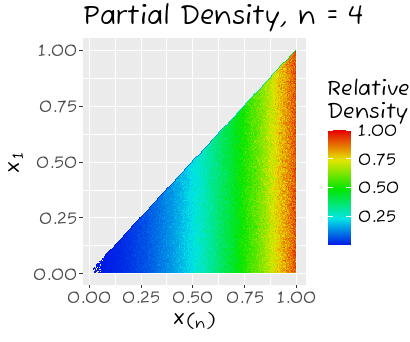
This description suggests several ways of depicting the distribution. First, to display the partial density, here is an empirical estimate of the partial density for $n=4$ based on a kernel density estimate from ten million samples.

(The colors on the diagonal $\Delta$ look slightly off because this graphic estimates densities by counting observations within tiny squares, but near $\Delta$ on the lower triangle of each square is occupied, resulting in an estimate that is only half as large as it should be.)
The vertical patterns of colors testify to the uniform distribution of $X_1$ conditional on $X_{(n)} = X_{n:n}.$
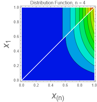
Next, here is a contour plot of the distribution function $F(t,s) = \Pr(X_{n:n}\lt t, X_1 \le s),$ also for $n=4:$

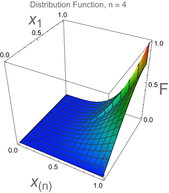
The jump across $\Delta$ is evident in the break in contour lines and fills. To help see this, here is a pseudo 3D plot of the same function.

Reference
Balakrishnan, N. and A. C. Cohen. Order Statistics and Inference (Estimation Methods). Academic Press, 1991.

