Please explain the waiting paradox

Question

A few years ago I designed a radiation detector that works by measuring the interval between events rather than counting them. My assumption was, that when measuring non-contiguous samples, on average I would measure half of the actual interval. However when I tested the circuit with a calibrated source the reading was a factor of two too high which meant I had been measuring the full interval.

In an old book on probability and statistics I found a section about something called "The Waiting Paradox". It presented an example in which a bus arrives at the bus stop every 15 minutes and a passenger arrives at random, it stated that the passenger would on average wait the full 15 minutes. I have never been able to understand the math presented with the example and continue to look for an explanation. If someone can explain why it is so that the passenger waits the full interval I will sleep better.

Answer 1

As Glen_b pointed out, if the buses arrive every $15$ minutes without any uncertainty whatsoever, we know that the maximum possible waiting time is $15$ minutes. If from our part we arrive "at random", we feel that "on average" we will wait half the maximum possible waiting time. And the maximum possible waiting time is here equal to the maximum possible length between two consecutive arrivals. Denote our waiting time $W$ and the maximum length between two consecutive bus arrivals $R$, and we argue that

$$ E(W) = \frac 12 R = \frac {15}{2} = 7.5 \tag{1}$$

and we are right.

But suddenly certainty is taken away from us and we are told that $15$ minutes is now the average length between two bus arrivals. And we fall into the "intuitive thinking trap" and think: "we only need to replace $R$ with its expected value", and we argue

$$ E(W) = \frac 12 E(R) = \frac {15}{2} = 7.5\;\;\; \text{WRONG} \tag{2}$$

A first indication that we are wrong, is that $R$ is not "length between any two consecutive bus-arrivals", it is "maximum length etc". So in any case, we have that $E(R) \neq 15$.

How did we arrive at equation $(1)$? We thought:"waiting time can be from $0$ to $15$ maximum. I arrive with equal probability at any instance, so I "choose" randomly and with equal probability all possible waiting times. Hence half the maximum length between two consecutive bus arrivals is my average waiting time". And we are right.

But by mistakenly inserting the value $15$ in equation $(2)$, it no longer reflects our behavior. With $15$ in place of $E(R)$, equation $(2)$ says "I choose randomly and with equal probability all possible waiting times that are smaller or equal to the average length between two consecutive bus-arrivals" -and here is where our intuitive mistake lies, because, our behavior has not change - so, by arriving randomly uniformly, we in reality still "choose randomly and with equal probability" all possible waiting times - but "all possible waiting times" is not captured by $15$ - we have forgotten the right tail of the distribution of lengths between two consecutive bus-arrivals.

So perhaps, we should calculate the expected value of the maximum length between any two consecutive bus arrivals, is this the correct solution?

Yes it could be, but : the specific "paradox" goes hand-in-hand with a specific stochastic assumption: that bus-arrivals are modeled by the benchmark Poisson process, which means that as a consequence we assume that the time-length between any two consecutive bus-arrivals follows an Exponential distribution. Denote $\ell$ that length, and we have that

$$f_{\ell}(\ell) = \lambda e^{-\lambda \ell},\;\; \lambda = 1/15,\;\; E(\ell) = 15$$

This is approximate of course, since the Exponential distribution has unbounded support from the right, meaning that strictly speaking "all possible waiting times" include, under this modeling assumption, larger and large magnitudes up to and "including" infinity, but with vanishing probability.

But wait, the Exponential is memoryless: no matter at what point in time we will arrive, we face the same random variable, irrespective of what has gone before.

Given this stochastic/distributional assumption, any point in time is part of an "interval between two consecutive bus-arrivals" whose length is described by the same probability distribution with expected value (not maximum value) $15$: "I am here, I am surrounded by an interval between two bus-arrivals. Some of its length lies in the past and some in the future but I have no way of knowing how much and how much, so the best I can do is ask What is its expected length -which will be my average waiting time?" - And the answer is always "$15$", alas.

Answer 2

If the bus arrives "every 15 minutes" (i.e. on a schedule) then the (randomly arriving) passenger's average wait is indeed only 7.5 minutes, because it will be uniformly distributed in that 15 minute gap.

--

If, on the other hand, the bus arrives randomly at the average rate of 4 per hour (i.e. according to a Poisson process), then the average wait is much longer; indeed you can work it out via the lack of memory property. Take the passenger's arrival as the start, and the time to the next event is exponential with mean 15 minutes.

Let me take a discrete time analogy. Imagine I am rolling a die with 15 faces, one of which is labelled "B" (for bus) and 14 labelled "X" for the total absence of bus that minute (fair 30 sided dice exist, so I could label 2 of the faces of a 30-sided die "B"). So once per minute I roll and see if the bus comes. The die has no memory; it doesn't know how many rolls since the last "B" it has been. Now imagine some unconnected event happens - a dog barks, a passenger arrives, I hear a rumble of thunder. From now, how long do I wait (how many rolls) until the next "B"?

Because of the lack of memory, on average, I wait the same time for the next "B" as the time between two consecutive "B"s.

[Next imagine I have a 60-sided die I roll every fifteen seconds (again, with one "B" face); now imagine I had a 1000-sided die I rolled every 0.9 seconds (with one "B" face; or more realistically, three 10-sided dice each and I call the result a "B" if all 3 come up "10" at the same time)... and so on. In the limit, we get the continuous time Poisson process.]

Another way to look at it is this: I am more likely to observe my 'start counting rolls' (i.e. 'the passenger arrives at the bus stop') event during a longer gap than a short one, in just the right way to make the average wait the same as the average time between buses (I mostly wait in long gaps and mostly miss out on the shortest ones; because I arrive at a uniformly distributed time, the chance of me arriving in a gap of length $t$ is proportional to $t$)

As a veteran catcher of buses, in practice reality seems to lie somewhere in between 'buses arrive on a schedule' and 'buses arrive at random'. And sometimes (in bad traffic), you wait an hour then 3 arrive all at once (Zach identifies the reason for that in comments below).

Answer 3

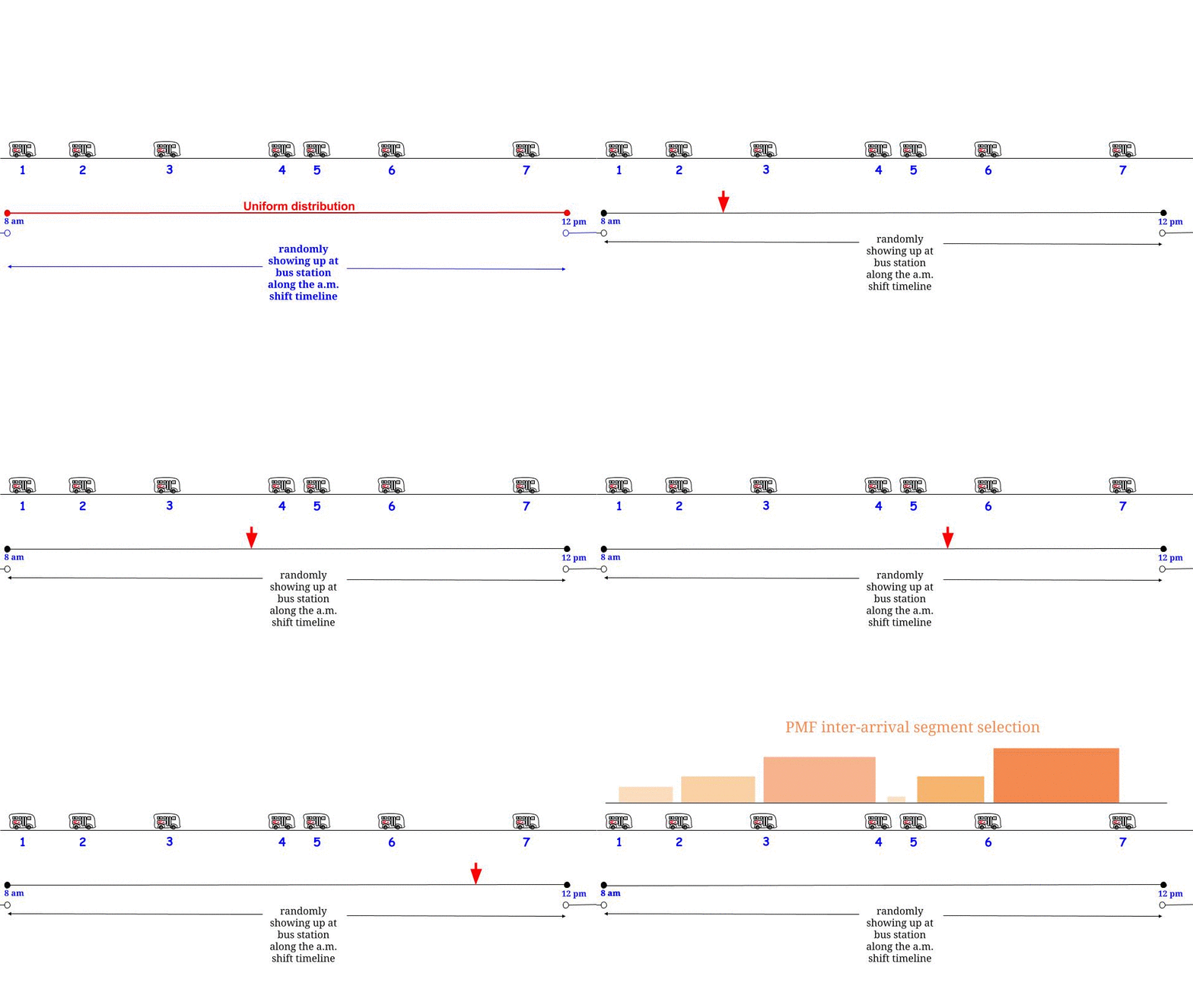
More on buses... Sorry to butt into the conversation so late in the discussion, but I have been looking at Poisson processes lately... So before it slips out of my mind, here is a pictorial representation of the inspection paradox:

The fallacy stems from the assumption that since buses follow a certain pattern of arrival with a given inter-arrival average time (the inverse of the Poisson rate parameter $\lambda$, let's call it $\small \theta=1/\lambda=15$ min.), by showing up at the bus station at any random time, you are in effect picking up a bus. So if you show up at the bus station at random times, keeping up a log-book of the waiting times over, say, one month, will actually give you the average inter-arrival time between buses. But this is not what you'd be doing.

If we were at a dispatch center, and could see all the buses on a screen, it would be true that randomly picking up multiple buses, and averaging the distance to the bus following behind, would produce the average inter-arrival time:

But, if what we instead do is just show up at the bus station (instead of selecting a bus), we are doing a random cross-section of time, say, along the timeline of the bus schedule in a typical morning. The time we decide to show up at the bus station may very well be uniformly distributed along the "arrow" of time. However, since there are longer time gaps between buses spread more farther apart, we are more likely to end up oversampling these "stragglers":

... and hence, our waiting time log book will not reflect the inter-arrival time. This is the inspection paradox.

As for the actual question on the OP regarding the expected waiting time of $15'$, minutes the mind-boggling explanation resides in the memoryless-ness of the Poisson process that makes the time-gap elapsed from the time the last bus we missed left the station to the time we show up irrelevant, and the expected time to the arrival of the next bus continues to be, stubbornly, $\theta=15$ minutes. This is best seen in discrete time (geometric distribution) with the dice example in Glen_b's answer.

In fact, if we could know how long ago the preceding bus left, the $\small \mathbb E[\text{time waiting (future) + time to last bus departure (past)}]=30$ min! As explaine in this MIT video by John Tsitsiklis, we just would have to view what precedes the point of arrival as a Poisson process backwards in time:

---

---

Still unclear? - try it with Legos.

Answer 4

There is a simple explanation which resolves the different answers which one gets from calculating expected waiting time for buses arriving per a Poisson Process with given mean interarrival time (in this case 15 minutes), whose interarrival times are therefore i.i.d. exponential with mean of 15 minutes.

Method 1) Because Poisson Process (exponential) is memoryless, the expected wait time is 15 minutes.

Method 2) You are equally likely to arrive at any time during the interarrival period in which you arrive. Therefore the expected waiting time is 1/2 of the expected length of this interarrival period. THIS IS CORRECT, and does not conflict with method (1).

How can (1) and (2) both be correct? The answer is that the expected length of the interarrival period for the time at which you arrive is not 15 minutes. It is actually 30 minutes; and 1/2 of 30 minutes is 15 minutes, so (1) and (2) agree.

Why does the interarrival period for the time at which you arrive not equal 15 minutes? It's because by first "fixing" an arrival time, the interarrival period it is in is more likely than average to be a long interarrival period. In the case of an exponential interarrival period, the math works outs so the interarrival period containing the time at which you arrive is an exponential with double the mean interarrival time for the Poisson Process.

It is not obvious that the exact distribution for the interarrival time containing the time at which you arrive would be an exponential with doubled mean, but it is obvious, after explanation, why it is increased. As an easy to understand example, let's say that the interarrival times are 10 minutes with probability 1/2 or 20 minutes with probability 1/2. In this case, 20 minutes long interarrival periods are equally likely to occur as 10 minute long interarrival periods, but when they do occur, they last twice as long. So, 2/3 of the time points during the day will be at times at which the interarrival period is 20 minutes. Put another way, if we first pick a time and then want to know what the interarrival time containing that time is, then (ignoring transient effects at the beginning of the "day") the expected length of that interarrival time is 16 1/3. But if we first pick the interarrival time and want to know what its expected length is, it is 15 minutes.

There are other variants of the renewal paradox, length-biased sampling, etc., amounting to pretty much the same thing.

Example 1) You have a bunch of light bulbs, with random lifetimes, but average of 1000 hours. When a light bulb fails, it is immediately replaced by another light bulb. If you pick a time to go in a room having the light bulb, the light bulb in operation then will wind up having a longer mean lifetime than 1000 hours.

Example 2) If we go to a construction site at a given time, then the mean time until a construction worker who is working there at that time falls off the building (from when they first started working) is greater than the mean time until worker falls off (from when they first started working) from among all workers who start working. Why, because the workers with a short mean time until falling off are more likely than average to have already fallen off (and not continued working), so that the workers who are working then have longer than average times until falling off.

Example 3) Pick some modest number of people at random in a city and if they have attended the home games (not all sell outs) of the city's Major League baseball team, find out how many people attended the games they were at. Then (under some slightly idealized but not too unreasonable assumptions), the average attendance for those games will be higher than the average attendance for all the team's home games. Why? Because there are more people who have attended high attendance games than low attendance games, so you are more likely to pick people who have attended high attendance games than low attendance games.

Answer 5

The question as posed was "...a bus arrives at the bus stop every 15 minutes and a passenger arrives at random." If the bus arrives every 15 minutes then its not random; it arrives every 15 minutes so the correct answer is 7.5 minutes. Either the source was incorrectly quoted or the writer of the source was sloppy.

On the other hand, the radiation detector sounds like a different problem because radiation events do arrive at random according to some distribution, presumably something like Poisson with an average waiting time.