Understand order of time series

Question

I am trying to build a time series model. I looked at the ACF/PACF and adf test of the series and thought that an ARMA(p,q) model will be suitable for the data. However when I run auto.arima(), it's showing the best model as ARMA(0,0). I am unable to understand how is this possible considering order 1 auto correlation to be 0.63. Attaching the acf/pacf plots . Appreciate any help on understanding the time series and suggestion on type of forecast model for this data. Thanks in advance

ADF Test : 
    Augmented Dickey-Fuller Test
Dickey-Fuller = -6.2373, Lag order = 13, p-value = 0.01
alternative hypothesis: stationary 

> auto.arima(ConvPCT)
Series: ConvPCT 
ARIMA(0,0,0) with non-zero mean 

Coefficients:
intercept  
 0.0191  

 sigma^2 estimated as 0.0002188:  log likelihood=6467.12
  AIC=-12932.24   AICc=-12932.23   BIC=-12920.74

if I run an ARMA(1,1) model, this is what I get

> Arima(ConvPCT,order=c(1,0,1))
Series: ConvPCT 
ARIMA(1,0,1) with non-zero mean 

Coefficients:
       ar1      ma1  intercept
       0.9633  -0.7048     0.0191
 s.e.  0.0076   0.0235     0.0018

sigma^2 estimated as 0.0001133:  log likelihood=7227.76
AIC=-14447.52   AICc=-14447.5   BIC=-14424.53

Here are two links for the same data file filesave link and wikiupload link. For model building, we can consider instances > 6% as outliers

Answer 1

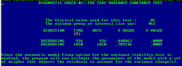
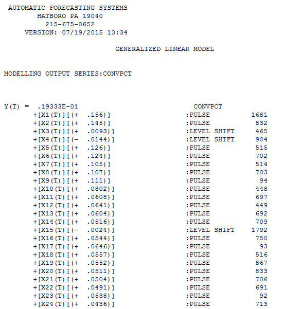
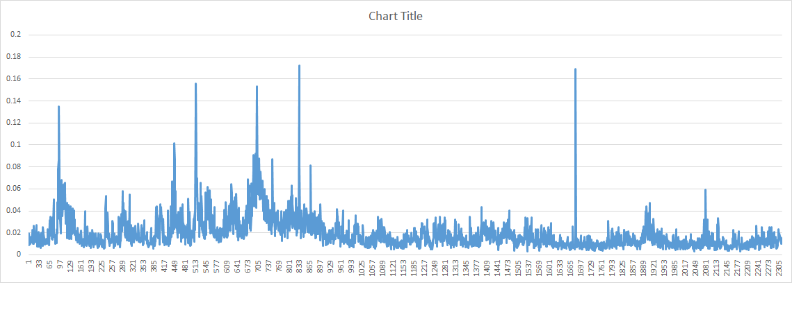
Parametric statistical tests often have unstated assumptions. For example the ADF test assumes no deterministic structure is present i.e. outliers/level shifts/seasonal pulses/time trends. The test also assumes invariant parameters over time. The test also assumes invariant error variance over time which is suspect given the plot of the data. Plots of data are often insufficient to identify assumption violations but in this case it is unusally informative. There is more than a hint of non-constant variance in the observed Y BUT the critical issue/assumption regards the constancy of the error variance from a reasonable model. I took your data and used AUTOBOX (my tool of choice), a commercial piece of software that I have helped develop to automatically analyze data. As surmised not only where there numerous pulses found but three points in time where the series changed level ( 465(+) , 904 (-) and 1792 (-) . Additionally a significant error variance reduction was detected at periods 926 and 1850 suggesting three regimes.

Following is a graph of the actual/fit and forecast 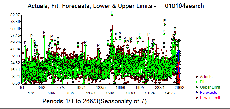. The variance change points were . The final model includes the 3 level shifts , a score of pulses and an AR(1) coefficient. Here are some model details ... and .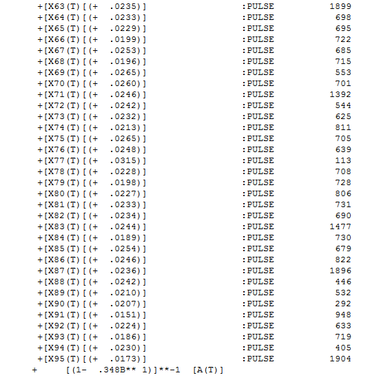

In summary the basic tools of ARIMA model identification make a lot of assumptions. Validating those assumptions and empirically identifying remedial action (pulses/level shifts/error variance breakpoints) culminates in what appears a satisfactory model. Unfortunately textbooks (even free on-line ones ) and very basic web tools are often inadequate to deal with the complexities you face with this data set. These are really not complexities but opportunities ! . The lessons from Ecclesiastes come to mind regarding when I was a child , simple tools were useful but as a man I need to use more powerful tools.....such is the advancement of science. Thanks for sharing this rather daunting time series with the group as there are lots of lessons to be learned here.

EDIT TO RESPOND TO COMMENT 1 and 2 :

The data is daily thus the seasonality is 7 as you have 7 readings per week. The transformation that is applied to Y is a weight derived from the significant change in variance that was detected at period 926 and 1850. In this case due to reducing error variance the whole idea here is that more recent values are more believable (less variability) and thus should have more weight. Non-constant error variance does not necessarily suggest the need for a power transform or a Garch transform as evidence of deterministic change points in error variance can be readily dealt with GLS (Generalized Least Squares) which essentially applies variance-stabilizing weights to the data. The actual weights used here for period 1-925 was .6 and for periods 926-1849 a .89 and for periods 1850-2314 a 1.0. These are computed from the two F values (.448.and .789 respectively ) . For example .89 is the square root of .789 .

YET ANOTHER EDIT TO RESPOND TO THREE COMMENTS

1&2) As you said the off-diagonal elements of the var-cov reflect the ar(1) structure while the diaonal elements reflect the non-constant error variance. These diagonal elements wotld reflect three regimes based upon the two f tests . What I was doing in my summary was to illustrate that adjusting the 2314 values for "degree of belief" was functionally equivalent to GLS where the elements on the diagonal were based upon the weights developed by TSAY but never put into a GLS persepctive , which was my small contribution . Using AUTOBOX there is no need to form the variance-covariance matrix but if you are employing functional computing alternatives then you cam develop that from the F values required to make the co-variance matrix of the residuals idempotent..

3) yes level is a dummy variable (0 before 1 at point ant thereafter )

historical pulses DON'T affect forecasts

don't know what you mean "through impulse response "

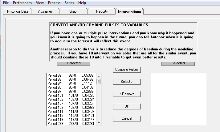
AUTOBOX presents the Intervention Variables based upon there order of importance however there is an additional report which presents them chronologically. I have shown a partial list.

[1-.348B**1] is the AR component which is a denominator polynomial on the error process thus the -1

If you wish you can contact me off line and I will try and help further as it sounds like you are very interested in my findings. I can be reached at 215-394-8897 if you would like more help.