6
$\begingroup$

I trying to implement the classic Monte-Carlo simulation of $\pi$ to better understand how confidence intervals (CI) decrease with more trials. There are a lot of examples of how to do the former, but I haven't been able to find a simple example of calculating the CI for it, and my method is producing CIs that seem too small to be accurate. Here's my approach:

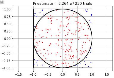
First, (using numpy) I draw $N$ random values between -1 and 1 in a uniform distribution to represent x and y coordinates. Then I calculate the radius of all points, find the number of points within a radius of 1, and calculate $\pi$ as the number of points within the circle, divided by $N$ multiplied by 4.

N = 500  # trials
X = np.random.uniform(-1, 1, N)
Y = np.random.uniform(-1, 1, N)
# Get radius of all points
rad_arr = np.sqrt((X ** 2) + (Y ** 2))
# Get boolean mask of points in circle
in_circle = rad_arr < 1.0  
pi_est = 4 * np.sum(in_circle) / N

Circle Viz

So far this is pretty standard and works perfectly. I'm now trying to understand how the confidence interval decreases as $N$ goes from 1 to 500. To do this I create the following array $\hat{\pi}_{est}$:

# Array of pi estimations from 1 to N
pi_est = 4 * np.cumsum(in_circle) / np.arange(1, N+1)

The array of the cumulative sum of points in the circle, divided by an array from 1 to $N$ creates an $N$-length array of the mean value of $\pi$ as $N$ goes from 1 to 500. Then I calculated an array of the corresponding 95% confidence interval with the following formula $1.96 \cdot \frac{\sigma_{\pi est_i}}{\sqrt{N_i}}$, where $\sigma_{\pi est_i}$ is the sample standard deviation for the estimate of $\pi$ at the $i$th step of N containing $N_i$:

N_arr = np.arange(N)
est_error = [1.96 * np.std(pi[:i]) / np.sqrt(i) for i in range(1, N+1)]
upper_ci = pi + est_error
lower_ci = pi - est_error

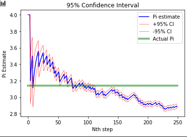
CI Viz

This last image looks really wrong. Specifically, the CI's are way to narrow at the beginning and not encompassing the actual value of $\pi$.

I have also tested a method where I draw $M$ draws of different $N$-point samples, so that each sample is independent from each other which produces better results:

M = 100
pi = np.zeros(M)
for i in range(M):
    N = i + 1  # trials
    X = np.random.uniform(-1, 1, N)
    Y = np.random.uniform(-1, 1, N)
    # Get radius of all points
    rad_arr = np.sqrt((X ** 2) + (Y ** 2))
    # Get boolean mask of points in circle
    in_circle = rad_arr < 1.0  
    pi[i] = 4 * np.sum(in_circle) / N

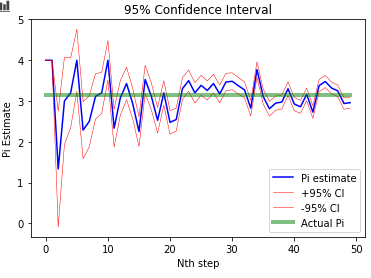
![CI Viz 2

But, the CIs still seem a little small to me, and I don't have a theoretical understanding of why this would work better then the previous method. The previous method also seems to be what all other examples of $\pi$ estimation via the Monte-Carlo method use (i.e Wikipedia's article on the Monte Carlo method).

Can someone explain what I'm doing wrong, and what I am misunderstanding about the Central Limit Theorem or sampling or CI calculation that is leading to this error?

---- UPDATE 1 ---

Based on suggestion by @EngrStudent, I've increased the sample size and did bootstrap resampling with replacement. Code:

M = 20000
X = np.random.uniform(-1, 1, M)
Y = np.random.uniform(-1, 1, M)
    
pi = np.zeros(M)
for i in range(M):
    N = i + 1  # trials
    _X = np.random.choice(X, size=N, replace=True) 
    _Y = np.random.choice(Y, size=N, replace=True)
    # Get radius of all points
    rad_arr = np.sqrt((_X ** 2) + (_Y ** 2))
    # Get boolean mask of points in circle
    in_circle = rad_arr < 1.0  
    pi[i] = 4 * np.sum(in_circle) / N

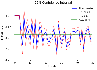
For the sake of legibility, I've cropped the image to the first 50 trials.

Here's my results with a sample size of 20,000:

enter image description here

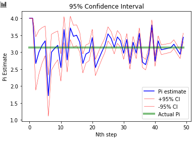
And here's one with 100,000:

enter image description here

I tried some different sample sizes, and it doesn't look to me like changing the sample size makes a difference, the CI's are looking more correct though. If this is correct, I'd still appreciate an explanation of the theory behind why this works!

$\endgroup$
10
  • 1
    $\begingroup$ Vastly too few samples. Start at around 20,000 and go up from there. That is going to engage the mean, not the variance. I would consider bootstrap resampling at the time-steps in order to estimate the interval. $\endgroup$ Commented May 20, 2021 at 4:12
  • 1
    $\begingroup$ @EngStudent, can you explain what you mean by boostrap resampling? Do you mean at every time step I resample from the N-length uniform distribution? If so, is this similar to what I'm doing in the second test I tried (running M trials where each N is sampled independently). Also what's the underlying theory of why this should work versus my incorrect method? $\endgroup$
    – saeranv
    Commented May 20, 2021 at 4:41
  • 1
    $\begingroup$ So the set up is you have had 100 points to put into the domain and used to estimate the pie. There are two ways to bootstrap it. The purest bootstrapping does not move any of the points. You would uniformly randomly select them based on index, and then re-compute. The second way would be to re-spread them in the domain and computer again. These two are going to have very different results. The second method will be much wider and represent the non-correlated estimate. $\endgroup$ Commented May 20, 2021 at 23:26
  • 1
    $\begingroup$ Thank you, now I understand. Also, in retrospect I think our whole conversation about sample size was backwards. Your intuition was correct. Looking at Thomas' throw number it seems like it takes 6e4 throws (or points) before the answer converges to second significant digit of Pi. However, my objective was to compute the standard error/CI, which should reflect the larger variance associated with smaller sample sizes. So the sample size is kind of irrelevant to this specific problem. Your second suggestion of bootstrapping (with "re-spreading") was the right answer though. $\endgroup$
    – saeranv
    Commented May 21, 2021 at 4:42
  • 1
    $\begingroup$ @EngrStudent well said. And just to be clear, I wasn't criticizing the suggestion to increase sample size, it provided a lot of insight to me about precision. I'm just trying to clarify why it was tangential since I myself was very confused about the role sample size had to play in determining better confidence intervals. $\endgroup$
    – saeranv
    Commented May 21, 2021 at 16:35

1 Answer 1

11
$\begingroup$

The standard error that you want is the standard deviation of the estimate $\hat\pi$ at a fixed point in the sequence, over multiple experiments. This standard error will give you a confidence interval that includes the actual value $\pi$ in 95% of experiments. You don't need a huge sample size to get reasonable estimation of the standard error; you need a huge sample size to get an accurate estimate of $\pi$.

I'm going to do the code in R; translating to Python is left as an exercise for the reader.

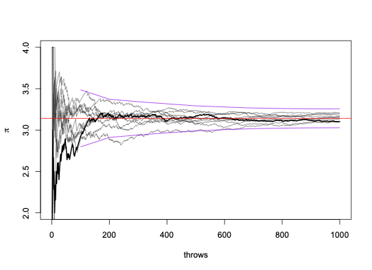
First, let's have a look at multiple runs: 100 runs of a 1000-step simulation

hatpi <- function(n){
    x <- runif(n)
    y<-runif(n)
    in_circle<- (x*x+y*y)<=1
    estimate_path<-4*cumsum(in_circle)/(1:n)
    estimate_path
}

plot(1:1000,hatpi(1000),type="l",lwd=2,ylab=expression(pi),xlab="throws",ylim=c(2,4))

for(i in 2:10){
    lines(1:1000,hatpi(1000),col="#00000080")
}
abline(h=pi,col="red")

enter image description here

You can see that the variation along each curve (which is what your first method uses) is smaller than the variation between the curves. That's because points on the same curve are correlated: the estimates at 800 and 900 throws share the first 800 throws and so have a correlation of 800/900, or nearly 0.9. Your standard error formula didn't take this into account

Now, I'll run a slightly larger set of experiments, 100, and estimate the standard deviation at 100,200,...,1000 throws

experiments<-matrix(0, ncol=10, nrow=100)
for(i in 1:100){
  one_experiment<-hatpi(1000)
  experiments[i,]=one_experiment[100*(1:10)]
}
stddevs <- apply(experiments,2,sd)
lines(100*(1:10), pi-1.96*stddevs,col="purple")
lines(100*(1:10), pi+1.96*stddevs,col="purple")

enter image description here

The standard deviations look more plausible now; the $\pm 1.96$ interval around the true value covers all 10 curves nearly all the way from 100 to 1000 (so the corresponding intervals around each curve would cover the true value).

We can actually do the calculations analytically here. The variance of the binary in_circle variable is $(\pi/4)\times(1-\pi/4)$, so the standard deviation of the estimate of $\pi$ based on $n$ throws is $4\sqrt{(\pi/4)\times(1-\pi/4)/n}$

truesd<-function(n) 4*sqrt((pi/4)*(1-pi/4)/n)

stddevs/truesd(100*(1:10))
 [1] 1.071722 1.015365 1.081009 1.090563 1.048619 1.043178 1.023968 1.042759 1.071379
[10] 1.115733

Even 100 experiments gave a reasonable estimate of the standard errors. Estimating the standard errors is relatively easy, because you'll probably be happy with the standard error being within about 10% of the truth, but you're trying to get $\pi$ to much more than one digit accuracy.

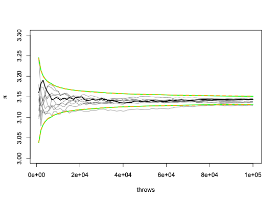
Now, a larger simulation: 1000 experiements with 100,000 throws each (but plotting only every 1000th throw)


experiments<-matrix(0, ncol=100, nrow=1000)
for(i in 1:1000){
  one_experiment<-hatpi(100000)
  experiments[i,]=one_experiment[1000*(1:100)]
}
stddevs <- apply(experiments,2,sd)

plot((1:100)*1000,experiments[1,],type="l",lwd=2,ylab=expression(pi),xlab="throws",ylim=c(3,3.3))
for(i in 2:10){
    lines(1000*(1:100),experiments[i,],col="#00000080")
}

lines(1000*(1:100), pi-1.96*stddevs,col="green",lwd=2)
lines(1000*(1:100), pi+1.96*stddevs,col="green",lwd=2)
lines(1000*(1:100), pi-1.96*truesd(1000*(1:100)),col="orange",lty=2,lwd=2)
lines(1000*(1:100), pi+1.96*truesd(1000*(1:100)),col="orange",lty=2,lwd=2)

enter image description here

I've only drawn 10 of the experiments, but you can still see the pattern. The estimated and analytic standard errors are almost identical (the green and orange curves are superimposed) and 9 of the 10 lines stay inside the interval.

The standard error is only 0.005 after 100,000 throws, so you'll need many more than that for a good value of $\pi$. The confidence intervals were well estimated with only 100 experiments, and 1000 experiments is overkill.

Finally, could you estimate the standard error from a single run? Yes, you could, but not the way you were doing it. Averages (and variances) of the binary in_circle variable along one run estimate the same thing as averages and variances across experiments. But averages and variances of the cumulative estimator don't -- they're increasingly correlated.

hatpi_with_sd<-function(n){
    x<-runif(n)
    y<-runif(n)
    in_circle<- (x*x+y*y)<=1
    estimate_path<-4*cumsum(in_circle)/(1:n)
    estimate_sd <-4*sd(in_circle)
    estimate_se <-estimate_sd/sqrt(1:n)
    list(estimate_path,estimate_se)
}

experiment<-hatpi_with_sd(1000)
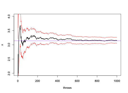
plot(1:1000,experiment[[1]],type="l",lwd=2,ylab=expression(pi),xlab="throws",ylim=c(2,4))
lines(1:1000, experiment[[1]]-1.96*experiment[[2]],col="red")
lines(1:1000, experiment[[1]]+1.96*experiment[[2]],col="red")
abline(h=pi,col="purple")

enter image description here

It works! The bootstrap idea is a slightly more general version of this, where the estimate_sd is based on empirical standard deviations over intervals of more than one time point, so it would work for, eg, autocorrelation estimates as well as for means.

$\endgroup$
9
  • $\begingroup$ Great answer! This has clarified a lot of theoretical and implementation confusion that I haven't been able to answer after days of looking online. I'm going to have to read it a couple more times to absorb the details, but this line alone "the estimates at 800 and 900 throws share the first 800 throws and so have a correlation of 800/900, or nearly 0.9" clarifies a lot. $\endgroup$
    – saeranv
    Commented May 20, 2021 at 7:18
  • $\begingroup$ I have some follow-up questions: In examples 2 and 3 where you're plotting the CIs for multiple experiments with 1000 and then 100,000 throws, why aren't you dividing the stddevs with the square root of the number of experiments at that point? I see pi-1.96*stddevs, but shouldn't it be pi-1.96*stddevs/range(1,experiment_number)? $\endgroup$
    – saeranv
    Commented May 20, 2021 at 7:27
  • $\begingroup$ Second question: You say that "Averages (and variances) of the binary in_circle variable along one run estimate the same thing as averages and variances across experiments." but wouldn't the correlation of in_circle at throw 800 and 900 also share the same first 800 points and thus have a correlation of 0.9? Why isn't this more correlated like the cumsum? $\endgroup$
    – saeranv
    Commented May 20, 2021 at 7:31
  • 1
    $\begingroup$ in_circle isn't correlated, it's just independent results of each throw. The reason not to scale stddevs by $1/\sqrt{n}$ is that it's already the standard deviation of the independent $\hat\pi$ estimates from different experiments, so it already gets smaller as they get closer together. $\endgroup$ Commented May 20, 2021 at 7:42
  • 1
    $\begingroup$ estimate_sd is the population sd of the individual throw estimates of $\pi$, which are either 4 or 0. estimate_se, which divides by sqrt(1:n) is the standard error of $\hat\pi$ after $n$ throws. $\endgroup$ Commented May 20, 2021 at 20:05

Your Answer

By clicking “Post Your Answer”, you agree to our terms of service and acknowledge you have read our privacy policy.

Not the answer you're looking for? Browse other questions tagged or ask your own question.