36
$\begingroup$

In this current article in SCIENCE the following is being proposed:

Suppose you randomly divide 500 million in income among 10,000 people. There's only one way to give everyone an equal, 50,000 share. So if you're doling out earnings randomly, equality is extremely unlikely. But there are countless ways to give a few people a lot of cash and many people a little or nothing. In fact, given all the ways you could divvy out income, most of them produce an exponential distribution of income.

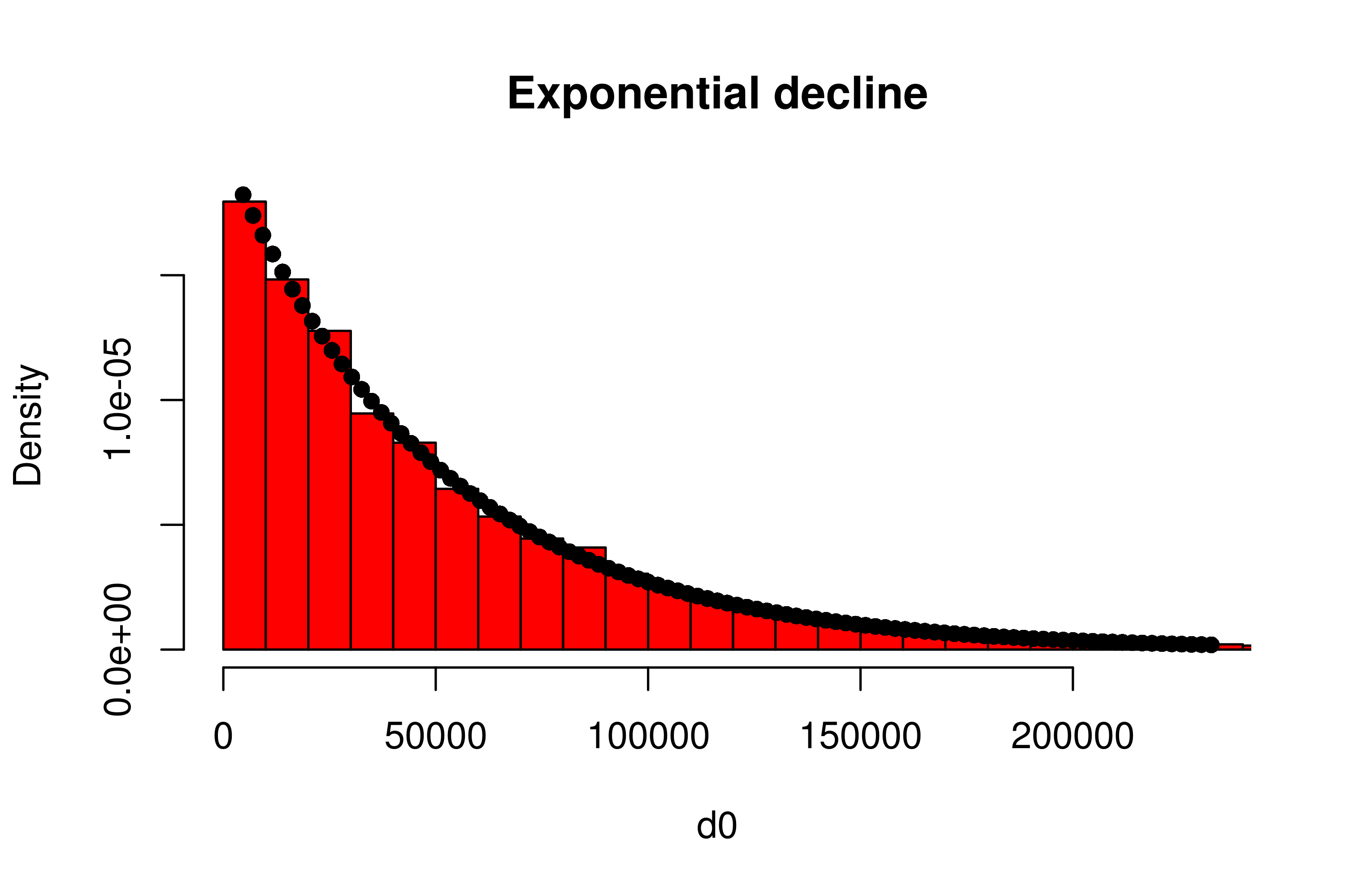
I have done this with the following R code which seems to reaffirm the result:

library(MASS)

w <- 500000000 #wealth
p <- 10000 #people

d <- diff(c(0,sort(runif(p-1,max=w)),w)) #wealth-distribution
h <- hist(d, col="red", main="Exponential decline", freq = FALSE, breaks = 45, xlim = c(0, quantile(d, 0.99)))

fit <- fitdistr(d,"exponential")
curve(dexp(x, rate = fit$estimate), col = "black", type="p", pch=16, add = TRUE)

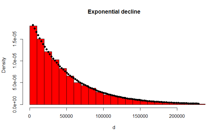
enter image description here

My question
How can I analytically prove that the resulting distribution is indeed exponential?

Addendum
Thank you for your answers and comments. I have thought about the problem and came up with the following intuitive reasoning. Basically the following happens (Beware: oversimplification ahead): You kind of go along the amount and toss a (biased) coin. Every time you get e.g. heads you divide the amount. You distribute the resulting partitions. In the discrete case the coin tossing follows a binomial distribution, the partitions are geometrically distributed. The continuous analogues are the poisson distribution and the exponential distribution respectively! (By the same reasoning it also becomes intuitively clear why the geometrical and the exponential distribution have the property of memorylessness - because the coin doesn't have a memory either).

$\endgroup$
8
  • 3
    $\begingroup$ If you give the money out one by one, there are many ways to distribute them evenly and many more to distribute them almost evenly (e.g. a distribution which is almost normal and with a mean of $50000$ and a standard deviation close to $224$) $\endgroup$
    – Henry
    Commented Sep 3, 2014 at 21:14
  • $\begingroup$ @Henry: Could you please describe this procedure a little bit more. Especially what do you mean by "one by one"? Perhaps you could even provide your code. Thank you. $\endgroup$
    – vonjd
    Commented Sep 4, 2014 at 14:29
  • $\begingroup$ vonjd: Start with 500 million coins. Allocate each coin independently and randomly between 10 thousand individuals with equal probability. Add up how many coins each individual gets. $\endgroup$
    – Henry
    Commented Sep 4, 2014 at 16:49
  • $\begingroup$ @Henry: The original statement was that most of the ways to distribute the cash yield an exponential distribution. Ways of distributing the cash and ways of distributing the coins are not isomorphic, since there is only one way to distribute \$500,000,000 uniformly among 10,000 people (give each \$50,000) but there are 500,000,000!/((50,000!)^10,000) ways of distributing 50,000 coins to each of 10,000 people. $\endgroup$
    – supercat
    Commented Sep 4, 2014 at 23:23
  • 1
    $\begingroup$ @Henry In the scenario you described in the uppermost comment, it is set from the beginning that each person has equal probability of getting the coin. This condition effectively assigns a huge weight to the normal distribution, rather than equally considering different ways to distribute the coins. $\endgroup$
    – higgsss
    Commented Sep 4, 2014 at 23:30

6 Answers 6

27
$\begingroup$

To make the problem simpler, let's consider the case where the allowed values of the share of each person is discrete, e.g., integers. Equivalently, one can also imagine partitioning the "income axis" into equally spaced intervals and approximating all values falling into a given interval by the midpoint.

Denoting the total income as $X$, the $s$-th allowed value as $x_{s}$, the total number of people as $N$, and finally, the number of people with shares of $x_{s}$ as $n_{s}$, the following conditions should be satisfied: \begin{equation} C_{1} (\{n_{s}\})\equiv\sum_{s} n_{s} - N = 0, \end{equation} and \begin{equation} C_{2} (\{n_{s}\})\equiv \sum_{s} n_{s} x_{s} - X = 0. \end{equation}

Notice that many different ways to divide the share can represent the same distribution. For example, if we considered dividing \$4 between two people, giving \$3 to Alice and \$1 to Bob and vice versa would both give identical distributions. As the division is random, the distribution with the maximum number of corresponding ways to divide the share has the best chance to occur.

To obtain such a distribution, one has to maximize \begin{equation} W(\{n_{s}\}) \equiv \frac{N!}{\prod_{s} n_{s}!}, \end{equation} under the two constraints given above. The method of Lagrange multipliers is a canonical approach for this. Furthermore, one can choose to work with $\ln W$ instead of $W$ itself, as "$\ln$" is a monotone increasing function. That is, \begin{equation} \frac{\partial \ln W}{\partial n_{s}} = \lambda_{1} \frac{\partial C_{1}}{\partial n_{s}} + \lambda_{2} \frac{\partial C_{1}}{\partial n_{s}} = \lambda_{1} + \lambda_{2} x_{s}, \end{equation} where $\lambda_{1,2}$ are Lagrange multipliers. Notice that according to Stirling's formula, \begin{equation} \ln n! \approx n\ln n - n, \end{equation} leading to \begin{equation} \frac{d\ln n!}{dn} \approx \ln n. \end{equation} Thus, \begin{equation} \frac{\partial \ln W}{\partial n_{s}} \approx -\ln n_{s}. \end{equation} It then follows that \begin{equation} n_{s} \approx \exp\big(-\lambda_{1} - \lambda_{2} x_{s}\big), \end{equation} which is an exponential distribution. One can obtain the values of Lagrange multipliers using the constraints. From the first constraint, \begin{equation} \begin{split} N &= \sum_{s} n_{s} \approx \sum_{s} \exp\big(-\lambda_{1} - \lambda_{2} x_{s}\big)\\ &\approx \frac{1}{\Delta x} \int_{0}^{\infty} \exp\big(-\lambda_{1} - \lambda_{2} x\big) \,\,dx\\ &=\frac{1}{\lambda_{2}\Delta x}\exp\big(-\lambda_{1}\big), \end{split} \end{equation} where $\Delta x$ is the spacing between allowed values. Similarly, \begin{equation} \begin{split} X &= \sum_{s} n_{s}x_{s} \approx \sum_{s} x_{s}\,\exp\big(-\lambda_{1} - \lambda_{2} x_{s}\big)\\ &\approx \frac{1}{\Delta x} \int_{0}^{\infty} x\,\exp\big(-\lambda_{1} - \lambda_{2} x\big) \,\,dx\\ &=\frac{1}{\lambda_{2}^{2}\,\Delta x}\exp\big(-\lambda_{1}\big). \end{split} \end{equation} Therefore, we have \begin{equation} \exp\big(-\lambda_{1}\big) = \frac{N^{2} \Delta x}{X}, \end{equation} and \begin{equation} \lambda_{2} = \frac{N}{X}. \end{equation} That this is really a maximum, rather than a minimum or a saddle point, can be seen from the Hessian of $\ln W - \lambda_{1} C_{1} - \lambda_{2} C_{2}$. Because $C_{1,2}$ are linear in $n_{s}$, it is the same as that of $\ln W$: \begin{equation} \frac{\partial^{2} \ln W}{\partial n_{s}^{2}} = -\frac{1}{n_{s}} < 0, \end{equation} and \begin{equation} \frac{\partial^{2} \ln W}{\partial n_{s}\partial n_{r}} = 0 \quad (s\neq r). \end{equation} Hence the Hessian is concave, and what we have found is indeed a maximum.

The function $W(\{n_{s}\})$ is really the distribution of distributions. For distributions we typically observe to be close to the most probable one, $W(\{n_{s}\})$ should be narrow enough. It is seen from the Hessian that this condition amounts to $n_{s}\gg 1$. (It is also the condition that Stirling's formula is reliable.) Therefore, to actually see the exponential distribution, partitions in the income axis (corresponding to bins in OP's histogram) should be wide enough so that number of people in a partition is much greater than unity. Towards the tail, where $n_{s}$ tends to zero, this condition is always destined to fail.

Note: This is exactly how physicists understand the Boltzmann distribution in statistical mechanics. The exponential distribution is essentially exact for this case, as we consider $N\sim 10^{23}$.

$\endgroup$
7
  • 1
    $\begingroup$ Thank you, please have a look at Glen_b's answer. Is this consistent with your answer? $\endgroup$
    – vonjd
    Commented Sep 3, 2014 at 11:01
  • 2
    $\begingroup$ @vonjd You're welcome! I think that his answer is consistent with mine. To me it seems that he is making an analogy to the Poisson process in the following sense: Consider a Poisson process with the "average time interval" of 50,000, and count 10,000 events. Then, on average, the "total time interval" is 50,000 x 10,000 = 500 million. $\endgroup$
    – higgsss
    Commented Sep 3, 2014 at 11:27
  • 2
    $\begingroup$ @vonjd I updated my answer. Most notably, I added the discussion on the condition that the distribution we typically observe is something close to the most probable distribution. $\endgroup$
    – higgsss
    Commented Sep 3, 2014 at 13:37
  • 2
    $\begingroup$ When considering discrete cases, would it be helpful to observe that T things can be divided among N people ((N+T-1) choose (N-1)) ways? If the first person receives f things, the number of ways one can distribute the remainder is ((N+T-f-2) choose (N-2)); the sum of that for values of f from 0 to N is the total number of ways of distributing everything. $\endgroup$
    – supercat
    Commented Sep 3, 2014 at 22:17
  • 1
    $\begingroup$ @supercat It looks like another way to derive the exponential distribution to me. Suppose that $T\gg N,f$ (we consider the values of $f$ that are not close to the tail of the distribution). Then, $(N+T-f-2)$ choose $(N-2) = (N+T-f-2)!/(N-2)!/(T-f)!$ $\propto (N+T-f-2)!/(T-f)! \approx (T-f)^{N-2} \approx T^{N-2} e^{-(N-2)f/T}$. $\endgroup$
    – higgsss
    Commented Sep 4, 2014 at 1:31
17
$\begingroup$

In fact you can prove it's not actually exponential, almost trivially:

Compute the probability that a given share is greater than $500$ million. Compare with the probability that an exponential random variable is greater than $500$ million.

However, it's not too hard to see that for your uniform-gap example that it should be close to exponential.

Consider a Poisson process - where events occur at random over along some dimension. The number of events per unit of the interval has a Poisson distribution, and the gap between events is exponential.

If you take a fixed interval then the events in a Poisson process that fall within it are uniformly distributed in the interval. See here.

[However, note that because the interval is finite, you simply can't observe larger gaps than the interval length, and gaps nearly that large will be unlikely (consider, for example, in a unit interval - if you see gaps of 0.04 and 0.01, the next gap you see can't be bigger than 0.95).]

So apart from the effect of restricting attention to a fixed interval on the distribution of the gaps (which will reduce for large $n$, the number of points in the interval), you would expect those gaps to be exponentially distributed.

Now in your code, you're dividing the unit interval by placing uniforms and then finding the gaps in successive order statistics. Here the unit interval is not time or space but represents a dimension of money (imagine the money as 50000 million cents laid out end to end, and call the distance they cover the unit interval; except here we can have fractions of a cent); we lay down $n$ marks, and that divides the interval into $n+1$ "shares". Because of the connection between the Poisson process and uniform points in an interval, the gaps in the order statistics of a uniform will tend to look exponential, as long as $n$ is not too small.

More specifically, any gap that starts in the interval placed over the Poisson process has a chance to be "censored" (effectively, cut shorter than it would otherwise have been) by running into the end of the interval.

$\hspace{1cm}$enter image description here
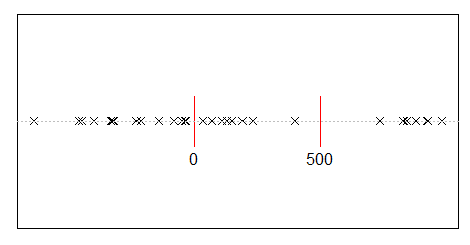
Longer gaps are more likely to do that than shorter ones, and more gaps in the interval means the average gap length must go down -- more short gaps. This tendency to be 'cut off' will tend to affect the distribution of longer gaps more than short ones (and there's no chance any gap limited to the interval will exceed the length of the interval -- so the distribution of gap size should decrease smoothly to zero at the size of the whole interval).

In the diagram, a longish interval at the end has been cut shorter, and a relatively shorter interval at the start is also shorter. These effects bias us away from exponentiality.

(The actual distribution of the gaps between $n$ uniform order statistics is Beta(1,n). )

So we should see the distribution at large $n$ look exponential in the small values, and then less exponential at the larger values, since the density at its largest values will drop off more quickly.

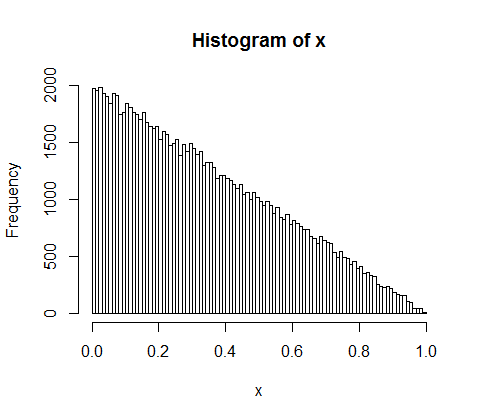
Here's a simulation of the distribution of gaps for n=2:
enter image description here

Not very exponential.

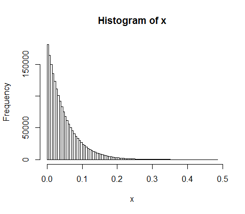
But for n=20, it starts to look pretty close; in fact as $n$ grows large it will be well approximated by an exponential with mean $\frac{1}{n+1}$.
enter image description here

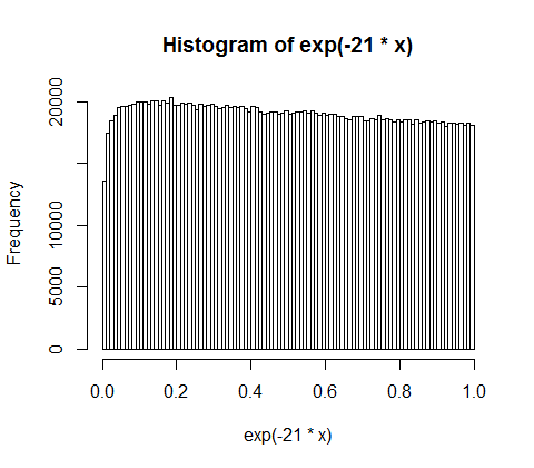
If that was actually exponential with mean 1/21, then $\exp(-21x)$ would be uniform... but we can see it isn't, quite:
enter image description here

The non-uniformity in the low values there corresponds to large values of the gaps -- which we'd expect from teh above discussion, because the effect of the "cutting off" the Poisson process to a finite interval means we don't see the largest gaps. But as you take more and more values, that goes further out into the tail, and so the result starts to look more nearly uniform. At $n=10000$, the equivalent display would be harder to distinguish from uniform - the gaps (representing shares of the money) should be very close to exponentially distributed except at the very unlikely, very very largest values.
$\endgroup$
7
  • 2
    $\begingroup$ So just to understand you correctly: You are saying that it is not exponential?!? higgsss proves above that it is exponential! $\endgroup$
    – vonjd
    Commented Sep 3, 2014 at 10:48
  • 3
    $\begingroup$ Let me quote my answer: (i) "you can prove it's not actually exponential" BUT (ii) for the uniform gaps you looked at "...it must be close to exponential" ... "as long as n is not too small." ... What's unclear? $\endgroup$
    – Glen_b
    Commented Sep 3, 2014 at 10:52
  • 5
    $\begingroup$ I outlined the (trivial, obvious) proof that it isn't actually exponential in my answer. higgss doesn't prove that it is exponential. That (excellent) answer is completely consistent with my statements. In it, higgsss proves that it will be approximately exponential: $n_{s} \approx \exp\big(-\lambda_{1} - \lambda_{2} x_{s}\big)$ $\endgroup$
    – Glen_b
    Commented Sep 3, 2014 at 10:55
  • 2
    $\begingroup$ I think that this answer is a great way to look at the problem, and deserves more upvotes. Yet I'm afraid that how the analogy to the Poisson process works (e.g., what "time" corresponds to) may appear unclear. Would you be willing give some more details? $\endgroup$
    – higgsss
    Commented Sep 3, 2014 at 11:13
  • 3
    $\begingroup$ @higgsss I've reworded slightly (removing reference to time), added a little detail and a link. I may add some more discussion later. If you have any specific suggestions, I'd be interested in improving my answer further. $\endgroup$
    – Glen_b
    Commented Sep 3, 2014 at 11:55
8
$\begingroup$

Let's suppose the money is infinitely divisible so we can deal with real numbers rather than integers.

Then the uniform distribution of $t=500000000$ partitioned across $n=10000$ individuals will give a marginal density for each individual $$p(x)=\frac{n-1}{t}\left(1-\frac{x}{t}\right)^{n-2}$$ for $0 \le x \le t$, and a marginal cumulative probability for each individual of $$P(X \le x)=1 - \left(1-\frac{x}{t}\right)^{n-1}.$$

If you want to apply this then use the marginal distribution to allocate a random amount $X$ to any of the individuals, then reduce $t$ to $t-X$ and $n$ to $n-1$ and repeat. Note that when $n=2$, this would give each individual a uniform marginal distribution across the remaining amount, much as one might expect; when $n=1$ you give all the remaining money to the single remaining person.

These expressions are polynomial rather than exponential, but for large $n$ you will probably find it hard to distinguish their effects from an exponential distribution with a parameter close to $\frac{n}{t}$. The distribution is asymptotically exponential because $\left(1-\frac{y}{m}\right)^{m} \to \exp(-y)$ as $m \to \infty$.

$\endgroup$
0
8
$\begingroup$

To say, "suppose you randomly divide 500 million in income among 10,000 people" is insufficiently specific to answer the question. There are many different random process that could be used to allocate a fixed amount of money to a fixed number of people, and each will have its own characteristics for the resulting distribution. Here are three generative processes I could think of, and the distributions of wealth each creates.

library(MASS)

w <- 500000000 #wealth
p <- 10000 #people

Method 1, posted by OP:

Choose 'p' numbers from [0,w) uniformly at random. Sort these. Append '0' to the front. Hand out dollar amounts represented by the differences between successive elements in this list.

d <- diff(c(0,sort(runif(p-1,max=w)),w)) #wealth-distribution
h <- hist(d, col="red", main="Exponential decline", freq = FALSE, breaks = 45,
     xlim = c(0, quantile(d, 0.99)))
fit <- fitdistr(d,"exponential")
curve(dexp(x, rate = fit$estimate), col = "black", type="p", 
      pch=16, add = TRUE)

uniform interval breaks

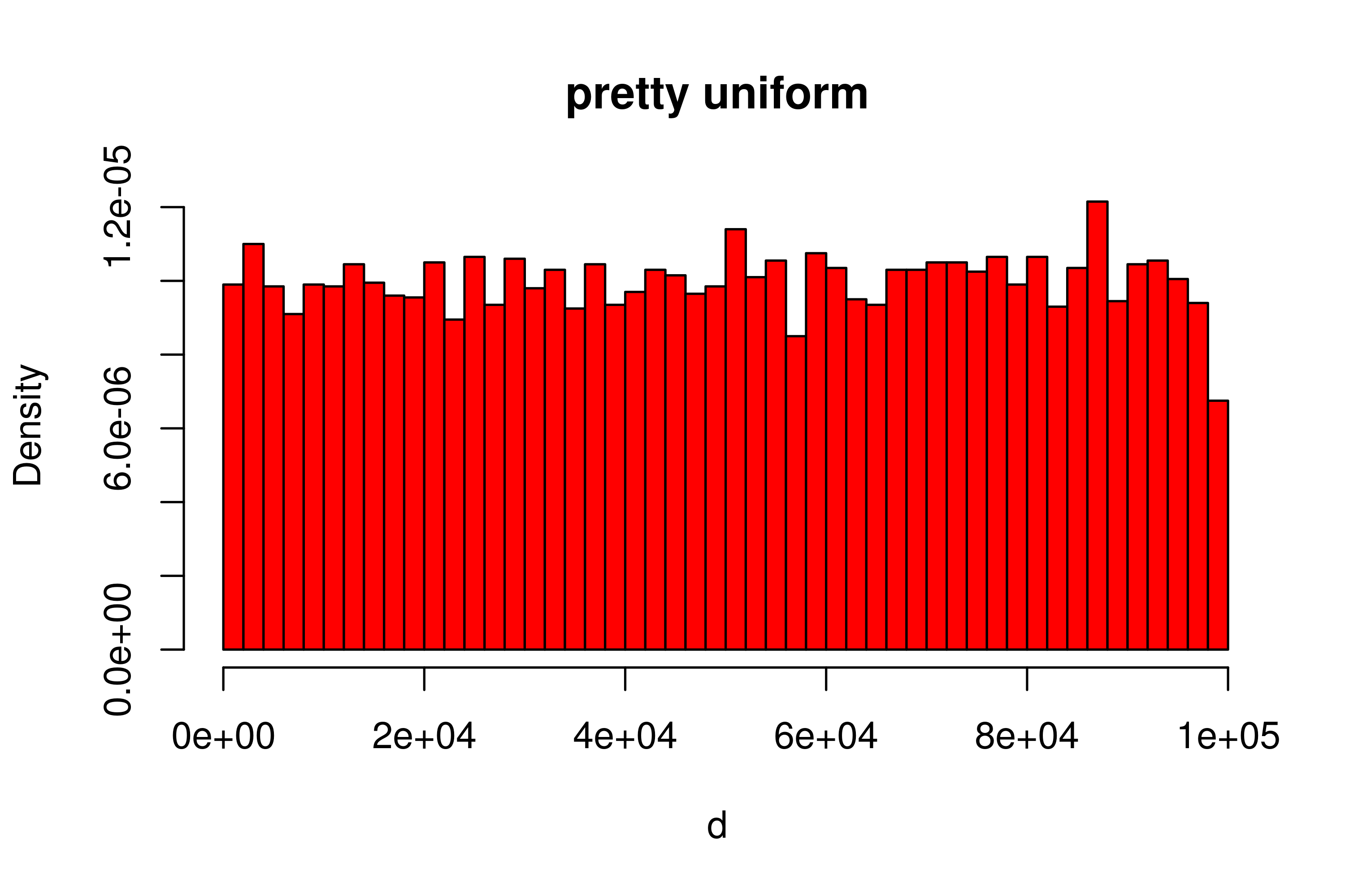
Method 2:

Chose 'p' numbers from [0, w) uniformly at random. Consider these 'weights', so 'w' doesn't actually matter at this stage. Normalize the weights. Hand out dollar amounts represented by the fraction of 'w' corresponding to each weight.

d <- runif(p,max=w) #weigh-distribution
d <- d/sum(d)*w #wealth-distribution
h <- hist(d, col="red", main="pretty uniform", freq = FALSE, breaks = 45, 
          xlim = c(0, quantile(d, 0.99)))

rescaled weights

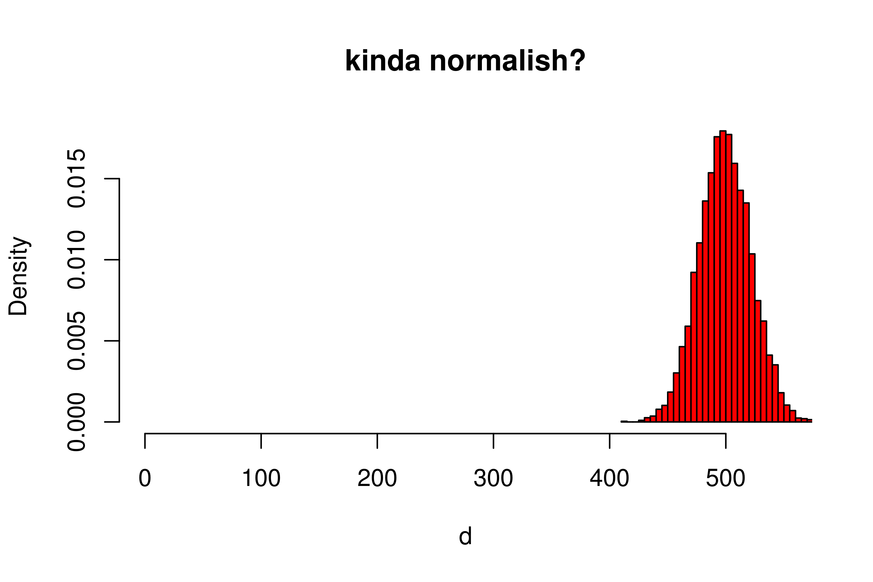
Method 3:

Start with 'p' 0s. w times, add 1 to a one of them, selected uniformly at random.

d <- rep(0, p)
for( i in 1:5000000){ ## for-loops in R are terrible, but this gives the idea.
    k <- floor(runif(1, max=p)) + 1    
    d[k] = (d[k] + 1)
}
h <- hist(d, col="red", main="kinda normalish?", freq = FALSE, breaks = 45,
          xlim = c(0, quantile(d, 0.99)))

iterative dollars

$\endgroup$
0
4
$\begingroup$

Let me add something regarding your addendum.

In the continuous case, as pointed out by Glen_b and Henry, the exact PDF for the amount each person receives is \begin{equation} p(x) = \frac{N-1}{X}\left(1-\frac{x}{X}\right)^{N-2}, \end{equation} where $N$ is the number of people, and $X$ is the total amount of money.

In the discrete case, assuming that there are $M$ coins to distribute, the probability for a particular person to receive $m$ coins is \begin{equation} p(m) = \frac{N-1}{M+1}\prod_{j=0}^{N-3}\left(1-\frac{m}{M-j}\right)^{N-2}. \end{equation} When $M\gg N$, two cases agree with each other. For sufficiently large $N$ and as long as we stay away from the tail, they look like exponential distributions.

In both cases, as we are sampling $N$ times from this true probability distribution, there will be error associated with the finite sample size.

However, performing the error analysis does not seem to be straightforward because different samplings in this case are not independent. They have to sum up to the total amount, and how much the first person receives affects the probability distribution for the second person, and so on.

My previous answer does not suffer from this issue, but I think it would be helpful to see how it can be resolved in this approach.

$\endgroup$
3
$\begingroup$

Good theoretical analysis done by the upvoted answers. However, here's my simple, empirical view on why the distribution is exponential.

When you distribute the money randomly, let's consider you do it one-by-one. Let S be the original sum.

For the first man, you must choose a random amount between 0 and S. Thus, on average, you will choose S/2 and remain with S/2.

For the second man, you would choose randomly between 0 and, on average, S/2. Thus, on average, you'll choose S/4 and remain with S/4.

So, you would basically be splitting the sum in half each time (statistically speaking).

Although in a real-life example you will not have continuously halved values, this shows why one should expect the distribution to be exponential.

$\endgroup$
3
  • 3
    $\begingroup$ Your algorithm tens to give more money to the first person than to any of the others. There are other approaches which do not have this bias. $\endgroup$
    – Henry
    Commented Sep 4, 2014 at 16:53
  • $\begingroup$ @Henry How else would you begin sharing the money? You must start with someone. And when you do, you have the whole amount in front of you. Giving him a random fraction literally means selecting at random from the entire sum. One cannot say that the assumption of having a "first man" is wrong, because otherwise the one who shares the money would simply divide the sum by the number of men since he knows in advance how many people there are. That's just my point of view: when you say you split the money "randomly", there will simply be one man getting more money $\endgroup$ Commented Sep 4, 2014 at 19:54
  • $\begingroup$ Bogdan Alexandru: My algorithm (another answer) has the feature that the distribution for each individual is the same no matter whether they are chosen first, in the middle or last. It also corresponds to a uniform density across the space constrained by the total amount being allocated. $\endgroup$
    – Henry
    Commented Sep 4, 2014 at 20:04

Your Answer

By clicking “Post Your Answer”, you agree to our terms of service and acknowledge you have read our privacy policy.

Not the answer you're looking for? Browse other questions tagged or ask your own question.