0
$\begingroup$

My question is how to perform TukeyHSD multiple comparison on ratio(for example, conversion rate, graduate school admit rate) using multcomp package in R. Take UCLA admission data for example:

mydata <- read.csv("http://www.ats.ucla.edu/stat/data/binary.csv")
mydata$rank <- factor(mydata$rank)

head(mydata)
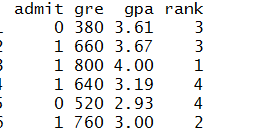
enter image description here

admit=1 means admitted. So if I am going to multi-pair comparison of admission rate(sum(admit)/count(admit)) between "rank", can I do it as what COOLSerdash proposed in the link: Comparing levels of factors after a GLM in R

mydata <- read.csv("http://www.ats.ucla.edu/stat/data/binary.csv")
mydata$rank <- factor(mydata$rank)
my.mod=glm(admit~rank, data=mydata,family=quasibinomial)
my.mod.mc=glht(my.mod, mcp(rank="Tukey"))
summary(my.mod.mc)
     Simultaneous Tests for General Linear Hypotheses

Multiple Comparisons of Means: Tukey Contrasts


Fit: glm(formula = admit ~ rank, family = quasibinomial, data = mydata)

Linear Hypotheses:
           Estimate Std. Error z value Pr(>|z|)    
2 - 1 == 0  -0.7500     0.3095  -2.423   0.0709 .  
3 - 1 == 0  -1.3647     0.3371  -4.049   <0.001 ***
4 - 1 == 0  -1.6867     0.4114  -4.100   <0.001 ***
3 - 2 == 0  -0.6147     0.2758  -2.229   0.1127    
4 - 2 == 0  -0.9367     0.3628  -2.582   0.0473 *  
4 - 3 == 0  -0.3220     0.3866  -0.833   0.8357  

If that's the case, how to interpret "Estimate" field?

thanks,

Kyle

$\endgroup$

2 Answers 2

1
$\begingroup$

I think it is OK to do what you did. You are simply comparing linear predictions from the model with an appropriate multiplicity adjustment, and if those are relevant to your study, then this does the trick.

To understand the estimate, note that it is on a scale that is the difference of two linear predictions, in this case with the default link function for quasibinomial, which is the logit (i.e., $\log[p/(1-p)]$ or the log odds ratio). A positive difference of two such values indicates that the first $p$ is greater than the second $p$. If you compute the $\exp$ function of these estimated differences, you obtain ratios of odds ratios. For instance, if the odds of one event are 2:1 and the odds of another are 4:1, then the ratio of these odds are $2/4=0.5$ and the difference of logits is $\log 0.5 \approx -0.693$.

$\endgroup$
2
  • $\begingroup$ for my own clarification, isn't what the OP asking different from what he is showing? He states he is going to calculate percentages but shows a linear model between the 'raw' data where admit is binomial. Are you saying he can replace 'admit' with 'admission rate' or is the linear model equivalent to evaluating 'admission rate'? $\endgroup$
    – cdeterman
    Commented Dec 15, 2014 at 13:36
  • $\begingroup$ Not totally sure what cdeterman is asking, but the model predicts logit(admission rate). $\endgroup$
    – Russ Lenth
    Commented Dec 15, 2014 at 14:22
1
$\begingroup$

If I am not mistaken, you actually want a chi square test as you are comparing population proportions. Taking the dataset you provide, you can easily make a contingency table in R.

tab <- table(mydata$admit, mydata$rank)
> tab

     1  2  3  4
  0 28 97 93 55
  1 33 54 28 12

You can then run a chi square analysis on this object with the chisq.test function. However, you must realize that you then should do post-hoc comparisons. In this case, running a chi square test on each pair of columns (i.e. ranks). Keep in mind with multiple comparisons you also need a correction such as bonferroni. Hopefully this can get you started.

$\endgroup$
1
  • 1
    $\begingroup$ Hi cdeterman,just out of curiosity, whats the difference between running a chi square test on each pair of columns and running a two proportion z-test? $\endgroup$
    – Kyle
    Commented Dec 14, 2014 at 7:04

Your Answer

By clicking “Post Your Answer”, you agree to our terms of service and acknowledge you have read our privacy policy.

Not the answer you're looking for? Browse other questions tagged or ask your own question.