If you stipulate three things, you can arrive at a definite answer:
The chance you are willing to accept that the prediction will be wrong if it is actually put to the test. 5%? 1%? Let's call this value $\alpha \gt 0$. $1-\alpha$ is the confidence of the prediction.
The number of different laboratories you use, $k$.
A distributional law for the chance variation.
As an illustration, I computed the answer for a 5% chance with one laboratory, assuming a normal distribution with 9.1% coefficient of variation. Letting $X$ represent the patient's observed INR (a random variable, normally distributed) and $Y$ represent the laboratory's result, it turns out there is a 100-5 = 95% chance that $Y$ will lie between $X/1.29$ and $1.29 X$, which is between $1.94$ and $3.23$ when $X = 2.5$. (People familiar with the normal distribution may be surprised at how wide that interval is: $\delta$ is $3.2$ times the CV!)
The computation is carried out as follows. Given the multiplicative nature of the CV, I sought limits for $Y$ in the form $X/(1+\delta)$ and $X(1+\delta)$, with $\delta \gt 0$ to be determined. Assumption (3) states that $X$ and $Y$ are independently distributed according to a Normal law with unknown mean $\mu$ and standard deviation $0.091 \mu$. Thus, we must solve the equation
$$P_{\mu}(X/(1+\delta) \le Y \le X(1+\delta)) = 1-\alpha.$$
This probability can be restated in terms of $X'=X/\mu$ and $Y'=Y/\mu$, which are independently normally distributed with mean $1$ and standard deviation $0.091$ simply by dividing through by $\mu$: this places the primes on $X$ and $Y$. That is, the unknown parameter $\mu$ plays no role in the calculation. We do all probability calculations using a Normal distribution of mean $1$ and standard deviation equal to the CV.
The probability can be numerically integrated (it's not available in any simple form) and used in a numeric root finder, yielding the results reported above.

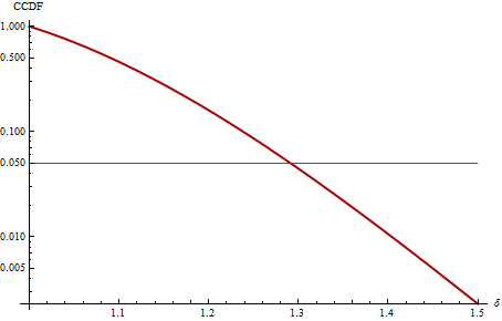
This plot shows, on a logarithmic scale in complementary cumulative distribution form (CCDF), the distribution of the ratio $\max(Y,X)/\min(Y,X)$ for a CV of 9.1%. For example, we can find $\alpha$ on the vertical axis and read across to find how extreme we can expect $1+\delta$ to be: about 1.3 for $\alpha = 0.05$, as shown previously. Conversely, we can take an observed ratio, such as 2.5/1.7 = 1.47 reported in an edit to the original equation, locate it on the horizontal axis, and read up (to a value of 0.005): this is the chance of observing a ratio this large. Because 0.005 is small, we would conclude (in this example) that interlaboratory variability (normally distributed, with CV of 9.1%) does not suffice to explain the difference between 1.7 and 2.5.
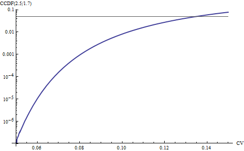
Note that the calculation is sensitive to the assumed CV. The next plot shows how the calculated chances vary with this assumption for CVs between 5% and 15%. For instance, if the true CV is really 13.5%, then observing a ratio of 2.5/1.7 or larger has a 5% chance of happening. Thus an alternative explanation of the pair (2.5, 1.7) is that variability actually is larger than expected (about 13.5/9.1 - 1 = 50% larger). If there are additional components of variability, such as changes in the subject over time, they could inflate the CV appreciably.

This approach to computing a prediction interval for $Y$ can be extended to compute prediction intervals for the maximum or minimum of $k$ additional independent realizations $Y_1, \ldots, Y_k$ when $k$ labs are used. The integrations are a little messier but the procedure is the same. Alternatively, we can use a Bonferroni-like adjustment by dividing the acceptable error $\alpha$ by $k$ and using that in the calculation: this tends to be a conservative, fairly accurate approximation in similar prediction interval situations (according to Hahn & Meeker, Statistical Intervals).
For example, still assuming a 5% error rate is acceptable, if you send samples to $k=4$ different laboratories for independent measurement, use $\alpha = 0.05/4 = 0.0125$ and find that $\delta = 0.389$, giving the range $[1.80, 3.47]$ for all four of the samples with 1-0.05 = 95% confidence.
Interpreting this result involves some subtleties. The chance computed here expresses a probability before any of the results are observed, even the one you have in hand ($X$, equal to 2.5 here). One can make a case that because we have already observed $X$, it is not random: it's a number. However, the approach described here takes the wider view as considered by the physician, not the patient. The physician needs to adopt a rational, fair procedure that works for many cases. Thus, the question s/he is asking is "as a policy, what general procedure should I establish to predict additional laboratory results $Y$ based on the initial readings $X$ I will be getting"? From this perspective, all the $X$s and all the subsequent $Y$s the physician will encounter in their practice truly are random and have not been observed. In the long run, we can be assured that by using this procedure, the physician can expect to err in the predictions only a fraction $\alpha$ of the time.
From the patient's point of view the question is a little different, because the patient is interested only in their particular case, not in the long run. A good solution for them might be to account for the special aspects of their situation and beliefs with a prior distribution for $X$, update that prior once $X$ is observed, and use the updated prior to predict the $Y$s. Whether or not this agrees with the general procedure here depends strongly on how consistent $X$ is with the prior: if it is consistent, the prediction interval will likely be narrower; but if it is not consistent, the two approaches could yield quite different answers.


