compute 95% confidence interval for predictions using a pooled model after multiple imputation?

Question

I am conducting multiple imputation by chained equations in R using the MICE package, followed by a logistic regression on the imputed dataset.

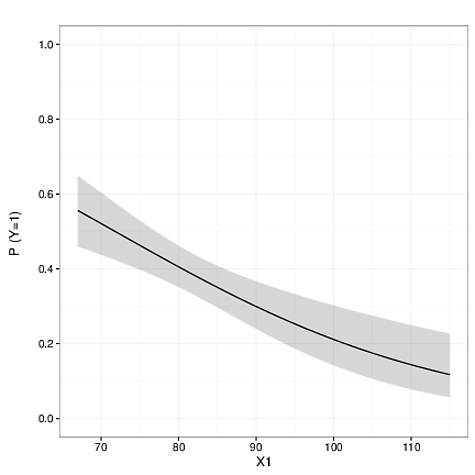
I need to compute a 95% confidence interval about the predictions for use in creating a plot—that is, the grey shading in the image below.

---

I followed the approach described in the answer to this question...

How are the standard errors computed for the fitted values from a logistic regression?

...which uses the following lines of code to yield the std.er of prediction for any specific value of the predictor:

o <- glm(y ~ x, data = dat)
C <- c(1, 1.5)
std.er <- sqrt(t(C) %*% vcov(o) %*% C)

But of course I need to adapt this code to the fact that I am using a model resulting from multiple imputation. In that context, I am not sure which variance-covariance matrix (corresponding to “vcov(o)” in the above example) I should be using in my equation to produce the "std.er".

---

Based on the documentation for MICE I see three candidate matrices:

• ubar - The average of the variance-covariance matrix of the complete data estimates.

• b - The between imputation variance-covariance matrix.

• t - The total variance-covariance matrix.

http://www.inside-r.org/packages/cran/mice/docs/is.mipo

Based on trying all three, the b matrix seems patently wrong, but both the t and the ubar matrices seem plausible. Can anybody confirm which one is appropriate?

Thank you.

Answer 1

The t matrix is the one to use in the way you describe. Eqs. 4 through 7 in the Dong & Peng paper that Joe_74 references correspond to the elements of the same names in the mipo object (documentation here), and so t is the accurate variance-covariance matrix for the pooled regression coefficients qbar you're actually using. ubar and b only matter here in that they are/were used to compute t.

Presumably you'll be using more than one predictor, so here's a MWE for that, which should be easy to modify.

set.seed(500)
dat <- data.frame(y = runif(20, 0, .5), x1 = c(runif(15),rep(NA, 5)), x2 = runif(20, 0.5))
imp <- mice(dat)
impMods <- with(imp, lm(y ~ x1 + x2))
pooledMod <- pool(impMods)
  # Generate some hypothetical cases we want predictions for
newCases <- data.frame(x1=c(4,7), x2=c(-6,0))
  # Tack on the column of 1's for the intercept
newCases <- cbind(1, newCases)
  # Generating the actual predictions is simple: sums of values times coefficients
yhats <- rowSums( sweep(newCases, 2, pooledMod$qbar, `*`) )
  # Take each new case and perform the standard operation
  # with the t matrix to get the pred. err.
predErr <- apply(newCases, 1, function(X) sqrt(t(X) %*% pooledMod$t %*% X))
  # Finally, put together a plot-worthy table of predictions with upper and lower bounds
  # (I'm just assuming normality here rather than using T-distribution critical values)
results <- data.frame(yhats, lwr=yhats-predErr*1.96, upr=yhats+predErr*1.96)

Answer 2

I recommend you to simply follow Rubin's rule, as spelled out in page 4 of this paper by Dong and Peng, SpringerPlus 2013:

http://www.ncbi.nlm.nih.gov/pmc/articles/PMC3701793/pdf/40064_2013_Article_296.pdf

Once you have obtained the variance, just proceed to the standard error (square root of the variance), and then use it to build the confidence interval using the t distribution with the correct degrees of freedom.

Answer 3

Perhaps something along the lines of extracting each of the fitted models from each of the imputed data sets, invoke predict on each of these and then bootstrap the results. The code below is laughably inefficient but may serve as a starting point for testing the idea. Additionally, there isn't really a need to compute the fitted values as you can obtain these directly from the pooled parameter estimates.

init = mice(df, maxit=0) 
meth = init$method  
predM = init$predictorMatrix

idat= mice(df, method=meth, predictorMatrix=predM, maxit = 20, m=10)
m1 <- with(idat, glm(adhered ~ age, family = binomial(link = "logit")))
summary(pool(m1))
newdata <- data.frame(age = seq(from = 25, to = 50, by = 1))

predictMI <- function(m, newdata, myseed = 12355){

  n.mods <- length(m$analyses)
  fit <- list()
  se <- list()

  for (i in 1:n.mods){

    mymod <- m$analyses[[i]]

    pred <- predict(mymod, 
                    newdata = newdata, 
                    type = "response", 
                    se = T)

    fit[[i]] <- pred$fit
	    se[[i]] <- pred$se
  }

  fit <- matrix(unlist(fit), ncol = n.mods, byrow = F)
  se <- matrix(unlist(se), ncol = n.mods, byrow = F)

  newdata$fit <- NA
  newdata$se <- NA
  set.seed(myseed)
  for (i in 1:nrow(newdata)){
    vals.fit <- fit[i,]
    vals.se <- se[i,]

    boot.res.fit <- vector()
    boot.res.se <- vector()
    for (j in 1:999){
      new.vals <- base::sample(vals.fit, length(vals.fit), replace = T)
      boot.res.fit[j] <- mean(new.vals)

      new.vals <- base::sample(vals.se, length(vals.se), replace = T)
      boot.res.se[j] <- mean(new.vals)
    }
    newdata$fit[i] <- mean(boot.res.fit)
	    newdata$se[i] <- mean(boot.res.se)
  }

  newdata$lwr <- newdata$fit - 1.96 * newdata$se
  newdata$upr <- newdata$fit + 1.96 * newdata$se
  newdata
}

Alternatively:

newdata <- data.frame(intercept = 1, age = seq(from = 25, to = 50, by = 1))
newdata <- as.matrix(newdata)
p1 <- pool(m1)
coefs <- p1$qbar

sigma <- p1$ubar
std.err <- vector()
for (i in 1:nrow(newdata)){
   C <- as.numeric(newdata[i,])
   std.err[i] <- sqrt(t(C) %*% sigma %*% C)  
}

mu <- newdata %*% matrix(coefs, ncol = 1)
invlogit <- function (x) {1/(1+exp(-x))}
newdata <- data.frame(newdata)
newdata$fit <- as.numeric(invlogit(mu))
newdata$lwr <- as.numeric(invlogit(mu - 1.96*std.err))
newdata$upr <- as.numeric(invlogit(mu + 1.96*std.err))


ggplot(data = newdata, aes(x = age, y = fit)) +
  geom_line() +
  geom_line(data = tes, aes(x = age, y = lwr), linetype = 2) +
  geom_line(data = tes, aes(x = age, y = upr), linetype = 2) +
  ylim(c(0,1))