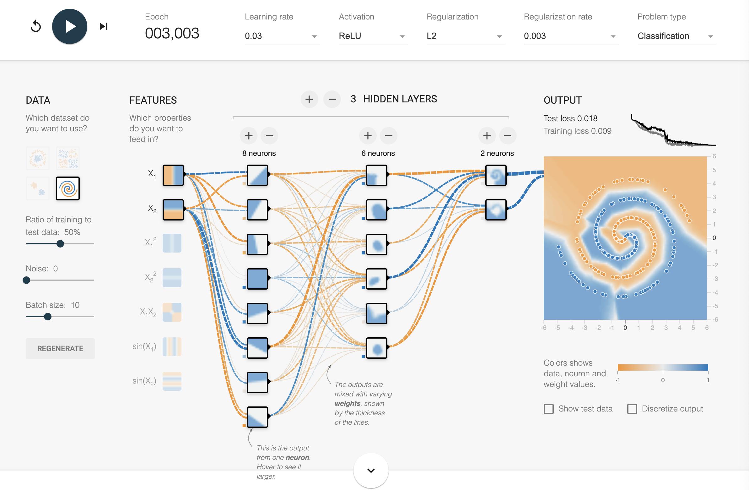
I have been messing around in tensorflow playground. One of the input data sets is a spiral. No matter what input parameters I choose, no matter how wide and deep the neural network I make, I cannot fit the spiral. How do data scientists fit data of this shape?
-
1$\begingroup$ Thank for the neat link, I had not seen this! Playing around quickly, from their default setup, if you just add the two "sin" features, it does a lot better. (Makes sense, as the spiral oscillates classes along any transect.) $\endgroup$– GeoMatt22Commented Sep 18, 2016 at 16:25
-
$\begingroup$ That was the first thing I tried but I got like 40-60% accuracy. $\endgroup$– Souradeep NandaCommented Sep 18, 2016 at 16:29
-
$\begingroup$ It seems to depend on the initialization a bit. I commonly got to 5% or so. (I think I took down the batch size to 5 also). You used sin(x) & sin(y) in addition to x & y? (this) $\endgroup$– GeoMatt22Commented Sep 18, 2016 at 16:33
-
1$\begingroup$ I should have just trained it a bit longer and used more neurons. It was actually trivially simple. $\endgroup$– Souradeep NandaCommented Sep 18, 2016 at 18:07
-
1$\begingroup$ AI: How to classify data which is spiral in shape? $\endgroup$– kenorbCommented Sep 19, 2016 at 18:52
4 Answers
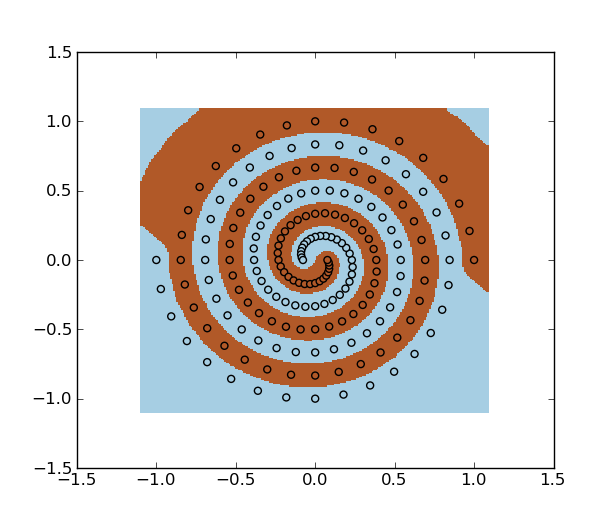
You could use SVM with an RBF kernel. Example:
import numpy as np
import matplotlib.pyplot as plt
import mlpy # sudo pip install mlpy
f = np.loadtxt("spiral.data")
x, y = f[:, :2], f[:, 2]
svm = mlpy.LibSvm(svm_type='c_svc', kernel_type='rbf', gamma=100)
svm.learn(x, y)
xmin, xmax = x[:,0].min()-0.1, x[:,0].max()+0.1
ymin, ymax = x[:,1].min()-0.1, x[:,1].max()+0.1
xx, yy = np.meshgrid(np.arange(xmin, xmax, 0.01), np.arange(ymin, ymax, 0.01))
xnew = np.c_[xx.ravel(), yy.ravel()]
ynew = svm.pred(xnew).reshape(xx.shape)
fig = plt.figure(1)
plt.set_cmap(plt.cm.Paired)
plt.pcolormesh(xx, yy, ynew)
plt.scatter(x[:,0], x[:,1], c=y)
plt.show()
You can also use least squares support vector machine.
spiral.data:
1 0 1
-1 0 -1
0.971354 0.209317 1
-0.971354 -0.209317 -1
0.906112 0.406602 1
-0.906112 -0.406602 -1
0.807485 0.584507 1
-0.807485 -0.584507 -1
0.679909 0.736572 1
-0.679909 -0.736572 -1
0.528858 0.857455 1
-0.528858 -0.857455 -1
0.360603 0.943128 1
-0.360603 -0.943128 -1
0.181957 0.991002 1
-0.181957 -0.991002 -1
-3.07692e-06 1 1
3.07692e-06 -1 -1
-0.178211 0.970568 1
0.178211 -0.970568 -1
-0.345891 0.90463 1
0.345891 -0.90463 -1
-0.496812 0.805483 1
0.496812 -0.805483 -1
-0.625522 0.67764 1
0.625522 -0.67764 -1
-0.727538 0.52663 1
0.727538 -0.52663 -1
-0.799514 0.35876 1
0.799514 -0.35876 -1
-0.839328 0.180858 1
0.839328 -0.180858 -1
-0.846154 -6.66667e-06 1
0.846154 6.66667e-06 -1
-0.820463 -0.176808 1
0.820463 0.176808 -1
-0.763975 -0.342827 1
0.763975 0.342827 -1
-0.679563 -0.491918 1
0.679563 0.491918 -1
-0.57112 -0.618723 1
0.57112 0.618723 -1
-0.443382 -0.71888 1
0.443382 0.71888 -1
-0.301723 -0.78915 1
0.301723 0.78915 -1
-0.151937 -0.82754 1
0.151937 0.82754 -1
9.23077e-06 -0.833333 1
-9.23077e-06 0.833333 -1
0.148202 -0.807103 1
-0.148202 0.807103 -1
0.287022 -0.750648 1
-0.287022 0.750648 -1
0.411343 -0.666902 1
-0.411343 0.666902 -1
0.516738 -0.559785 1
-0.516738 0.559785 -1
0.599623 -0.43403 1
-0.599623 0.43403 -1
0.65738 -0.294975 1
-0.65738 0.294975 -1
0.688438 -0.14834 1
-0.688438 0.14834 -1
0.692308 1.16667e-05 1
-0.692308 -1.16667e-05 -1
0.669572 0.144297 1
-0.669572 -0.144297 -1
0.621838 0.27905 1
-0.621838 -0.27905 -1
0.551642 0.399325 1
-0.551642 -0.399325 -1
0.462331 0.500875 1
-0.462331 -0.500875 -1
0.357906 0.580303 1
-0.357906 -0.580303 -1
0.242846 0.635172 1
-0.242846 -0.635172 -1
0.12192 0.664075 1
-0.12192 -0.664075 -1
-1.07692e-05 0.666667 1
1.07692e-05 -0.666667 -1
-0.118191 0.643638 1
0.118191 -0.643638 -1
-0.228149 0.596667 1
0.228149 -0.596667 -1
-0.325872 0.528323 1
0.325872 -0.528323 -1
-0.407954 0.441933 1
0.407954 -0.441933 -1
-0.471706 0.341433 1
0.471706 -0.341433 -1
-0.515245 0.231193 1
0.515245 -0.231193 -1
-0.537548 0.115822 1
0.537548 -0.115822 -1
-0.538462 -1.33333e-05 1
0.538462 1.33333e-05 -1
-0.518682 -0.111783 1
0.518682 0.111783 -1
-0.479702 -0.215272 1
0.479702 0.215272 -1
-0.423723 -0.306732 1
0.423723 0.306732 -1
-0.353545 -0.383025 1
0.353545 0.383025 -1
-0.272434 -0.441725 1
0.272434 0.441725 -1
-0.183971 -0.481192 1
0.183971 0.481192 -1
-0.0919062 -0.500612 1
0.0919062 0.500612 -1
1.23077e-05 -0.5 1
-1.23077e-05 0.5 -1
0.0881769 -0.480173 1
-0.0881769 0.480173 -1
0.169275 -0.442687 1
-0.169275 0.442687 -1
0.2404 -0.389745 1
-0.2404 0.389745 -1
0.299169 -0.324082 1
-0.299169 0.324082 -1
0.343788 -0.248838 1
-0.343788 0.248838 -1
0.373109 -0.167412 1
-0.373109 0.167412 -1
0.386658 -0.0833083 1
-0.386658 0.0833083 -1
0.384615 1.16667e-05 1
-0.384615 -1.16667e-05 -1
0.367792 0.0792667 1
-0.367792 -0.0792667 -1
0.337568 0.15149 1
-0.337568 -0.15149 -1
0.295805 0.214137 1
-0.295805 -0.214137 -1
0.24476 0.265173 1
-0.24476 -0.265173 -1
0.186962 0.303147 1
-0.186962 -0.303147 -1
0.125098 0.327212 1
-0.125098 -0.327212 -1
0.0618938 0.337147 1
-0.0618938 -0.337147 -1
-1.07692e-05 0.333333 1
1.07692e-05 -0.333333 -1
-0.0581615 0.31671 1
0.0581615 -0.31671 -1
-0.110398 0.288708 1
0.110398 -0.288708 -1
-0.154926 0.251167 1
0.154926 -0.251167 -1
-0.190382 0.206232 1
0.190382 -0.206232 -1
-0.215868 0.156247 1
0.215868 -0.156247 -1
-0.230974 0.103635 1
0.230974 -0.103635 -1
-0.235768 0.050795 1
0.235768 -0.050795 -1
-0.230769 -1e-05 1
0.230769 1e-05 -1
-0.216903 -0.0467483 1
0.216903 0.0467483 -1
-0.195432 -0.0877067 1
0.195432 0.0877067 -1
-0.167889 -0.121538 1
0.167889 0.121538 -1
-0.135977 -0.14732 1
0.135977 0.14732 -1
-0.101492 -0.164567 1
0.101492 0.164567 -1
-0.0662277 -0.17323 1
0.0662277 0.17323 -1
-0.0318831 -0.173682 1
0.0318831 0.173682 -1
6.15385e-06 -0.166667 1
-6.15385e-06 0.166667 -1
0.0281431 -0.153247 1
-0.0281431 0.153247 -1
0.05152 -0.13473 1
-0.05152 0.13473 -1
0.0694508 -0.112592 1
-0.0694508 0.112592 -1
0.0815923 -0.088385 1
-0.0815923 0.088385 -1
0.0879462 -0.063655 1
-0.0879462 0.063655 -1
0.0888369 -0.0398583 1
-0.0888369 0.0398583 -1
0.0848769 -0.018285 1
-0.0848769 0.018285 -1
0.0769231 3.33333e-06 1
-0.0769231 -3.33333e-06 -1
I had similar experiments comparing to Franck's answer. Please check this post.
Do all machine learning algorithms separate data linearly?
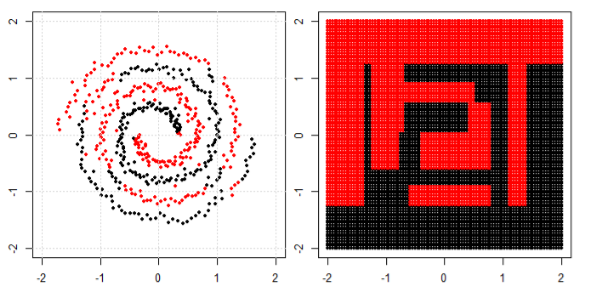
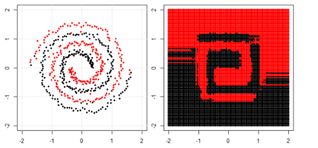
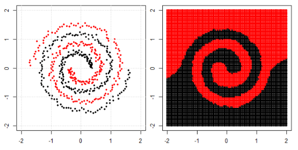
In the post we use tree, boosting and K nearest neighbor on spiral data.
KNN is most intuitive one, it make the classification according to a given point's neighbors. So, spiral data would not "break the neighbor rule"
For tree and boosting model, you can understand it as a "really complicated model that can achieve complied decisions". That is why you can see it can roughly learn the pattern, with some errors.
Finally you may search for special clustering or kernel PCA in google to see how can we deal with "connected components".
-
$\begingroup$ Funny thing about the tensorflow playground in terms of linear separation: The spiral is their only case that is not linearly separable! So if all of their input features are allowed, no hidden layers are required to classify their other data. (Of course there are interesting things to do using deeper networks when only a subset of the inputs are given.) $\endgroup$ Commented Sep 19, 2016 at 18:43
-
$\begingroup$ @GeoMatt22 in fact i haven't pay attention about OP's question on tensorflow playground... I think NN is powerful to do a lot of things. it cannot work well with the spiral data is because the the limitation of the web based tools? $\endgroup$ Commented Sep 19, 2016 at 18:48
-
$\begingroup$ The tensorflow playground app can do the spiral fine (in my comments to OP I link to one simple solution from r/MachineLearning). I think when doing their experiments that the OP was mostly just not patient enough in waiting for training to converge. $\endgroup$ Commented Sep 19, 2016 at 18:54
For this dummy problem you can increase the number of features. One particular way that I found to work is using extreme learning machines. Basically, you create a random matrix $K$ with columns equal to number of old features, $d$, and rows equal to number of new features $d'$(I had to use $d'=300d$). Also, create a random bias vector $b$ with length equal to $d'$. And you need a non-linear activation function $f$. Relu in particular works well --- $Relu(X) = max(X,0)$. Then perform linear logistic regression on the new data $X'=f(XK+b)$ (sloppy numpy or matlab notation for adding $b$ to every row of $XK$).
Here is a small code using the linear logistic regression of scikit-learn in python.
import numpy as np
import matplotlib.pyplot as plt
import sklearn.linear_model


f = np.loadtxt("spiral.data")
x, y = f[:, :2], f[:, 2]
new_feature_ratio = 300;
def relu(Y): return np.maximum(Y, 0)
cls = sklearn.linear_model.LogisticRegression(
    penalty='l2', C=1000, max_iter=1000)
K = np.random.randn(x.shape[1], x.shape[1]*new_feature_ratio)
b = np.random.randn(x.shape[1]*new_feature_ratio)
cls.fit( relu(np.matmul(x,K) + b) ,y)
xmin, xmax = x[:,0].min()-0.1, x[:,0].max()+0.1
ymin, ymax = x[:,1].min()-0.1, x[:,1].max()+0.1
xx, yy = np.meshgrid(np.arange(xmin, xmax, 0.01), np.arange(ymin, ymax,    0.01))
xnew = np.c_[xx.ravel(), yy.ravel()]
ynew = cls.predict(relu(np.matmul(xnew,K) + b)).reshape(xx.shape)
fig = plt.figure(1)
plt.set_cmap(plt.cm.Paired)
plt.pcolormesh(xx, yy, ynew)
plt.scatter(x[y>0,0], x[y>0,1], color='r')
plt.scatter(x[y<0,0], x[y<0,1], color='g')
plt.show()
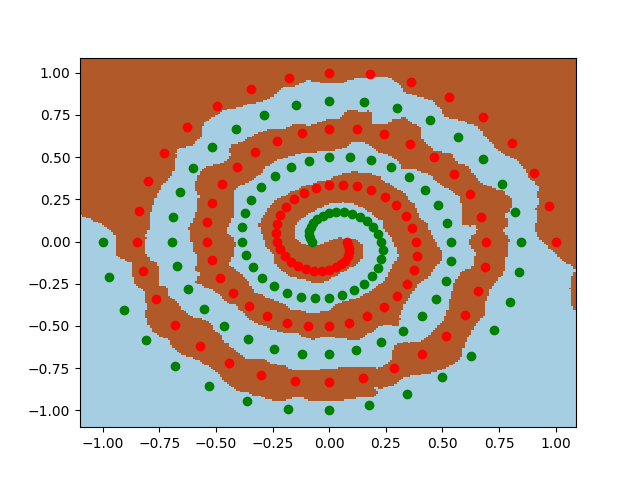
spiral.data is the same as Frank's answer. This strategy is basically a neural network where the first layer is chosen randomly rather than being trained.
You won't experience a "spiral" in the real world. But it is one of the more complex yet easy to visualize non-linear datasets. The playground in your question is for building intuition with neural networks. The other answers gave solutions that work but in my opinion miss the point of what can be learned here.
In the real world, most non-linear functions span complex hyperdimensional spaces that are impossible to directly visualize. Some intuition behind that here. While there are standard techniques to attempt to represent higher dimensional spaces such as t-SNE and more new ones like the Grand Tour you'll rarely be so lucky as to know ahead of time what the underlying function is. Even if you were, you likely wouldn't be able to manually engineer a sophisticated enough kernel that is generalizable enough.
What you do know is that neural networks are good universal approximators. A spiral dataset is merely a convenient tool to demonstrate just how difficult it can be to turn theory into reality. Some notes on systematic approaches to approximate a function with a neural network: A Recipe for Training Neural Networks and Machine Learning Yearning.
Following some of those methods, I was able to get the answer in about 30 minutes. I encourage people reading to try to arrive at it on their own first. It's a good analogy for the pain of training models in the real world. :)
Here's a solution that should get you to ~0.02 test loss/training loss by epoch 3000 using just the raw X1/X2 inputs. Solution

