Relationship between two time series: ARIMA

Question

Given the following two time series (x, y; see below), what is the best method to model the relationship between the long-term trends in this data?

Both time series have significant Durbin-Watson tests when modelled as a function of time and neither are stationary (as I understand the term, or does this mean it only needs to be stationary in the residuals?). I have been told that this means I should take a first-order difference (at least, maybe even 2nd order) of each time series before I can model one as a function of the other, essentially utilising an arima(1,1,0), arima(1,2,0) etc.

I don't understand why you need to detrend before you can model them. I understand the need to model the auto-correlation, but I don't understand why there needs to be differencing. To me, it appears as though detrending by differencing is removing the primary signals (in this case the long-term trends) in the data that we are interested in and leaving the higher-frequency "noise" (using the term noise loosely). Indeed, in simulations where I create an almost perfect relationship between one time series and another, with no autocorrelation, differencing the time series gives me results that are counterintuitive for relationship detection purposes, e.g.,

a = 1:50 + rnorm(50, sd = 0.01)
b = a + rnorm(50, sd = 1)
da = diff(a); db = diff(b)
summary(lmx <- lm(db ~ da))

In this case, b is related strongly with a, but b has more noise. To me this shows that differencing doesn't work in an ideal case for detecting relationships between low frequency signals. I understand that differencing is commonly used for time-series analysis, but it appears to be more useful for determining relationships between high-frequency signals. What am I missing?

Example Data

df1 <- structure(list(
x = c(315.97, 316.91, 317.64, 318.45, 318.99, 319.62, 320.04, 321.38, 322.16, 323.04, 324.62, 325.68, 326.32, 327.45, 329.68, 330.18, 331.08, 332.05, 333.78, 335.41, 336.78, 338.68, 340.1, 341.44, 343.03, 344.58, 346.04, 347.39, 349.16, 351.56, 353.07, 354.35, 355.57, 356.38, 357.07, 358.82, 360.8, 362.59, 363.71, 366.65, 368.33, 369.52, 371.13, 373.22, 375.77, 377.49, 379.8, 381.9, 383.76, 385.59, 387.38, 389.78), 
y = c(0.0192, -0.0748, 0.0459, 0.0324, 0.0234, -0.3019, -0.2328, -0.1455, -0.0984, -0.2144, -0.1301, -0.0606, -0.2004, -0.2411, 0.1414, -0.2861, -0.0585, -0.3563, 0.0864, -0.0531, 0.0404, 0.1376, 0.3219, -0.0043, 0.3318, -0.0469, -0.0293, 0.1188, 0.2504, 0.3737, 0.2484, 0.4909, 0.3983, 0.0914, 0.1794, 0.3451, 0.5944, 0.2226, 0.5222, 0.8181, 0.5535, 0.4732, 0.6645, 0.7716, 0.7514, 0.6639, 0.8704, 0.8102, 0.9005, 0.6849, 0.7256, 0.878),
ti = 1:52), 
.Names = c("x", "y", "ti"), class = "data.frame", row.names = 110:161)

ddf<- data.frame(dy = diff(df1$y), dx = diff(df1$x))
ddf2<- data.frame(ddy = diff(ddf$dy), ddx = diff(ddf$dx))
ddf$ti<-1:length(ddf$dx); ddf2$year<-1:length(ddf2$ddx)
summary(lm0<-lm(y~x, data=df1))      #t = 15.0
summary(lm1<-lm(dy~dx, data=ddf))    #t = 2.6
summary(lm2<-lm(ddy~ddx, data=ddf2)) #t = 2.6

Answer 1

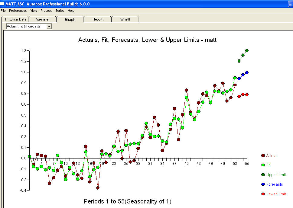
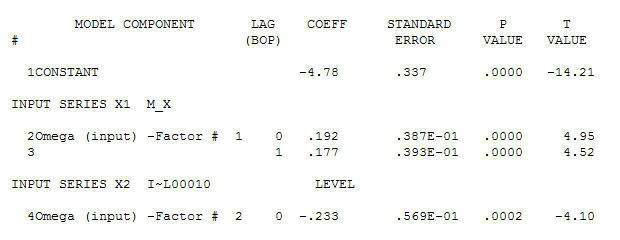Matt, You are very right in the concerns that you have raised with respect to using unnecessary differencing structure . In order to identify an appropriate model for your data yielding significant structure while rendering a Gaussian Error process 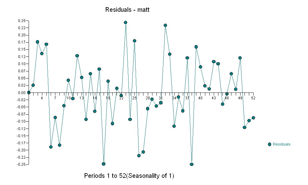with an ACF of 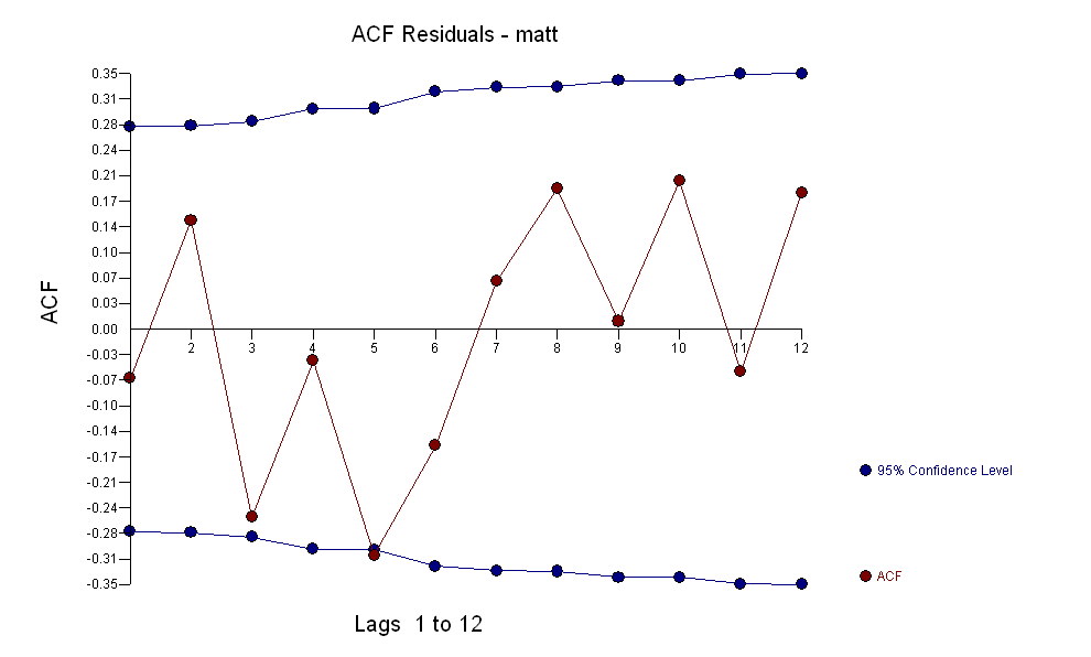the Transfer Function Identification modelling process requires ( in this case ) suitable differencing to create surrogate series that are stationary and thus usable to IDENTIFY the relationshop. In this the differencing requirements for IDENTIFICATION were double differencing for the X and single differencing for the Y. Additionally an ARIMA filter for the doubly differenced X was found to be an AR(1). Applying this ARIMA filter ( for identification purposes only ! ) to both stationary series yielded the following cross-correlative structure . suggesting a simple contemporaneous relationship. 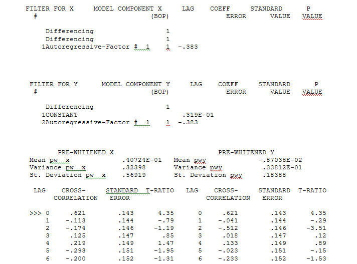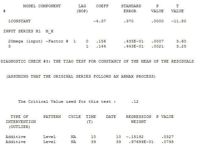. Note that while the original series exhibit non-stationarity this does not necessarily imply that differencing is needed in a causal model. 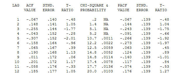The final model 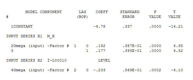and final acf support this . 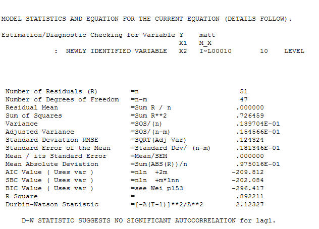In closing the final equation aside from the one empirically identified level shifts ( really intercept changes ) is

 Y(t)=-4.78 + .192*X(t) - .177*X(t-1) which is NEARLY equal to 

 Y(t)=-4.78 + .192*[X(t)-X(t-1)] which means that changes in X effect the level of Y

Finally note the characteristics of the suggested model.

the Level Shift series (0,0,0,0,0,0,0,0,0,1,1,.........,1) suggests if left untreated the model residuals would exhibit a level shift at or around time period 10 THUS a test of the hypothesis of a common residual mean between the first 10 residuals and the last 42 would be significant at alpha=.0002 based upon a "t test of -4.10" . Note that the inclusion of a constant guarantees that the overall mean of the residuals does not differ significantly from zero BUT this is not necessarily for all subset time intervals. The following graph clearly shows this ( given that you were told to look ! ).The Actual/Fit/Forecast is quite illuminating . Statistics are like lampposts, some use them to lean on others use them for illumination.

Answer 2

I don't understand that advice either. Differencing removes polynomial trends. If the series are similar because of the trends differencing essentially removes that relationship. you would only do that if you expect the detrended components to be related. If the same order of differencing leads to acfs for the residuals that look like they could be from a stationary ARMA model including white noise that may indicate that both series have the same or similar polynomial trends.

Answer 3

The way I understand it, differentiating gives clearer answers in the cross-correlation function. Compare ccf(df1$x,df1$y) and ccf(ddf$dx,ddf$dy).