Mixed effects model for power analysis to aid study design

Question

I am planning a study and would like to perform a power analysis to design the optimal sampling strategy. I would like to know how samples would be necessary to detect a significant effect.

The study is to assess whether there is a significant effect of habitat type on the growth rate of a species of snake. We will be collecting and measuring the length of snakes from three habitats (riverine, woodland, grassland). We expect that a snakes age will be the strongest predictor of its length. We have a way to estimate snake age to include this information in the model.

Data collected will look something like this:

Sample  length(cm)  Age(years)  Habitat
Snake1  30 3 Riverine
Snake2  43 5 Riverine
Snake3  10 1 Woodland  
Snake4  15  2 grassland

So to model if we will have power to detect an effect of habitat on the growth rate I believe I want to do a generalized mixed effect model. I want to see the effect of a categorical variable (habitat) on growth rate. I am unsure about the correct way to model this as I am only measuring snake length but it is growth rate that I am actually trying to learn, which is the slope of age and length.

I am not very familiar with generalized mixed models. From what I have been reading would it be appropriate to run two mixed models, one with and one without habitat as a predictor variable and then use an ANOVA to compare the two models to see if habitat has a significant effect on the response variable? I do not want the model to assume that growth rate is linear in each habitat, as the growth curve is something that may vary between habitats that we are also interested to measure. This is how I have it formulated so far but as I do not yet fully understand the model I suspect this is not correct:

Model 1: Length ~ (1 + age | habitat) + age

Model 2: Length ~ (1 | habitat) + age

Then ANOVA(Model 1, Model 2)

I would greatly appreciate any assistance with formulating an appropriate model for answering this question. Once I have a model I presume I can play around with generating simulated input data with different assumptions about the effect of habitat on growth rate and then change the sample sizes to see how many snakes I would need to measure to achieve a significant result.

It would be great to know if we assume a difference in growth rate of approximately 1cm per year how many snakes we would need to measure to detect this.

Answers that use R are welcome though I would be most interested in conceptually understanding how to formulate the correct model to address this question. Thank you in advance for your assistance.

Answer 1

Mixed-effects models may be explained in multiple ways. In your example, you could think of them as a way of accounting for variance explainable by some categorical variable (such as habitat) without paying the parameter penalty of including the variable as a fixed effect.

Suppose you had 20 different habitat types. You would have 19 implicit parameters in a regular modelling framework, while in a mixed-effects model you would be accounting for a single variance term (i.e. you would assume that the means of all 20 habitats are drawn from some normal distribution).

Now to get to the specifics of your case: since you have only 3 habitats, you don't really pay much of a penalty (2 parameters!). And 3 units is a very small number for estimating a variance term in any case. So I actually suggest that you abandon the mixed-effects modelling framework here and include 'habitat' as a fixed effect. This leaves you with a simple linear model:

Length ~ Age * Habitat

A strong interaction term would be clear evidence for your biological hypothesis of growth rate being influenced by habitat, I think. And if you know how to do a regular power analysis, you can go ahead and do this instead of worrying about the complexities of power analysis in mixed models (for which there are methods, e.g. http://onlinelibrary.wiley.com/doi/10.1111/2041-210X.12504/full).

Let me know if this addresses your question; I will try to clarify anything above that isn't clear, or point you towards additional resources.

EDIT in reply to your comment:

Answering your questions in reverse order

1) The simple linear model example I gave above will allow for different slopes in different habitats. That's what the interaction term essentially is. If you leave out an interaction term, you will force all slopes to be the same.

2) If you expand beyond 4-5 groups AND you do not care about making statistical comparisons between pairs of groups (which is probably not worth it), then you should almost certainly switch to a mixed modelling framework. In which case, the model you need would be your model 1 above, i.e.

Length ~ Age + (1 + Age | Habitat)

Statistically testing whether your random slope term is significant is trickier, but I believe the RLRsim package lets you do this (I have not tried it, but the authors know their stuff). The simR package I linked to above will let you do the mixed model power analyses relatively easily.

Answer 2

I have a pretty involved solution that requires you specify some hyperparameters of your model. Not being an expert in the relation between snake length and age, I picked some values that seemed vaguely possible. But, by all means feel free to tweak them. This series of functions is adapted and expanded from Gelman and Hill (2007).

First, we need a function to simulate data sets with the properties you want. Here is where I "invented" some numbers (under the comment #Specifying hyperparameters. Feel free to adjust accordingly based on your knowledge base and expectations.

#Creating fake dataframe for simulations 
fake<-function(J, K){
  snake<-(1:(J*K))          #creates a snake or case id 
  habitat<-rep(1:J, K)      #creates a balanced grouping variable   
  age<-rnorm(J*K, 2.5, .75) #creates a random normal age variable 
  #Specifying hyperparameters 
  mu.a.true<-12 #grand intercept 
  mu.g1.true<-3 #grand age slope 
  sigma.y.true<-1.65        #residual sd 
  sigma.a.true<-2.30        #intercept sd
  sigma.g1.true<-2.15       #age slope sd 
  #habitat-level parameters 
  a.true<-rnorm(J, mu.a.true, sigma.a.true) #vector of random intercepts
  g1.true<-rnorm(J, mu.g1.true, sigma.g1.true) #vector of random slopes  
  #dependent variable 
  y<-rnorm(J*K, a.true[habitat]+g1.true[habitat]*age, sigma.y.true)
  return(data.frame(snake, y, habitat, age))
}

and if you run print(fake(5,5)) you get the following simulated data (where y = length):

> print(fake(5,5))
   snake        y habitat       age
1      1 21.85790       1 1.9030948
2      2 27.73040       2 2.4382916
3      3 11.60743       3 0.7640231
4      4 15.63832       4 2.9965471
5      5 26.83866       5 1.8319489
6      6 24.65482       1 3.0666732
7      7 27.42804       2 2.2352739
8      8 16.98225       3 3.5354592
9      9 15.32236       4 3.0284722
10    10 25.22085       5 2.4662031
11    11 18.39988       1 2.2474545
12    12 21.85225       2 1.2652154
13    13 14.12972       3 2.6137810
14    14 17.69987       4 1.3900062
15    15 33.13150       5 3.2806024
16    16 28.80915       1 4.6216763
17    17 35.61110       2 2.5738612
18    18 15.78296       3 2.5815051
19    19 17.76041       4 3.2101400
20    20 29.23588       5 2.5638092
21    21 21.51020       1 2.7942239
22    22 32.10491       2 2.6981291
23    23 10.05619       3 1.7800981
24    24 16.96727       4 3.0558285
25    25 34.61646       5 3.3928710

Up next? We need to simulate a bunch of data and see how many data sets "recover" a significant effect for age given the hyperparameters we input in our data simulation function. Again, those hyperparameters can be adjusted to better fit your expectations.

mixed.power<-function(J, K, n.sims=1000){
  signif<-rep(NA, n.sims) #note that you can specify number of simulations - default is 1000
  pb<-winProgressBar(title="Progress", min=0, max=100, width=300)    #if you want to watch the progress
  require(lme4)
  require(arm)
  for(s in 1:n.sims){
    fake.data<-fake(J, K)                                               #calls in data simulation function
    lme.power<-lmer(y~1+age+(1+age|habitat), data=fake.data)            #estimates mixed effect model using each simulated dataset
    theta.hat<-fixef(lme.power)["age"]                                  #saves age coefficients from each simulated dataset 
    theta.se<-se.fixef(lme.power)["age"]                                #saves standard error of age coefficients from each simulated dataset
    signif[s]<-ifelse((abs(theta.hat)-qt(.975, J*K-1)*theta.se)>0, 1, 0)#assigns value of 1 to significant coefficients 0 to ns coefficients
    setWinProgressBar(pb, s/n.sims*100, title=paste(round(s/n.sims*100, 0), "% done"))
  }
  close(pb)
  power<-mean(signif, na.rm=T)#calculates proportion of significant models out of # of simulated datasets... 
  return(power)
}

You may get some warnings with these codes when models don't converge in your simulations. I find that happens more often when dealing with small samples like the ones you are proposing. (I tend to ignore these convergence warnings)

You can pause here and calculate power for a given number of habitats (J) with a given number of snakes per habitat (K), based on the parameters you specified above. In that case you can run mixed.power(5,10) and see the following returned:

> mixed.power(5, 10)
[1] 0.804

Or perhaps more instructively you can go all out and create a power plot to get a sense of how many snakes per habitat you should consider gathering. Here is the function for that:

graph.power<-function(J, max.K){
  require(ggplot2)
  KK<-seq(3, max.K, by=1)       #will ieterate from 3 cases to the max.K specified in the function above
  Y<-rep(NA, length(KK))        #Empty vector to contain power estimates from mixed.power () function
  JJ<-rep(J, length(KK))        #Repeates the number of habitats you specified to equal the length of the KK vector 
  pb2<-winProgressBar(title="Overall Progress", min=0, max=100, width=300)  #for an overall progress bar
  for(i in 1:length(KK)){
    Y[i]<-mixed.power(JJ[i], KK[i]) #runs mixed power function and stores results one at a time
    setWinProgressBar(pb2, i/length(KK)*100, title=paste(round(i/length(KK)*100, 0), "% Overall complete"))
  }
  close(pb2)
  DF<-as.data.frame(cbind(KK, Y)) #creates data frame for plotting
  colnames(DF)<-c("KK", "Y")
  #Code below provides a basic power plot with a horizontal line at .80 
  g1<-ggplot(aes(x=KK, y=Y), data=DF) 
  g2<-g1+geom_smooth(se=F)+geom_hline(yintercept = .8, lty="dashed", col="red", lwd=2)
  g3<-g2+xlab("Sample Size per Habitat")+ylab("Power")
  g4<-g3+ggtitle("Power Analysis")
  return(g4)
}

When you use this function, the only difference is that now the second number is the maximum number of snakes you want to consider examining in a power analysis. So in this example, let's say I wanted to look at a power curve that considered up to 15 snakes per habitat (holding the number of habitats constant at 5). Here is what that would look like: graph.power(5,15)... which would return the following image:

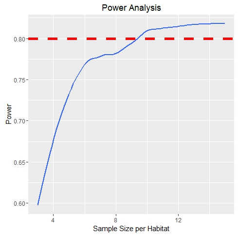
Now you have the ability to assess the sample size at which the power curve crosses .80 (~9 snakes per 5 habitats in this case).

This is NOT the only way to approach a power analysis in a mixed model, but I tend to like it as it gives me a great deal of control over the various hyperparameters and allows me to plot various power curves to get a sense of how changing those hyperparameters in addition to sample and cluster size change the power of my model.

A note: if you want to play around to get a sense of how the functions work or to try to identify some good starting values you may want to lower the number of simulations in the mixed.power() function to reduce computation time prior to running your "official" power analyses with the larger set of simulated data sets.