Aside from the heavily technical definitions of Brownian motion, the simplest is that if you run Brownian motion from a starting point $B_0=x$, the resulting distribution $B_t$ at time $t$ is Gaussian, with mean $x$ and variance $t$. This is useful because it gives you a sense of how spread out Brownian motion will be after time $t$, relative to a starting point $x$.
Concerning quadratic variation, this is primarily defined as a tool for evaluating integrals involving Brownian motion. Typical integrals looks like $\int_0^t f(t,B_t)dB_t$ or even simpler, $\int_0^t f(B_t)dB_t$ . Heuristically, you can evaluate this integral numerically by taking a small partition $[t_0=0,t_1,...,t_n,t_{n+1}=t]$ of $[0,t]$:
$$\int_0^tf(B_t)dB_t\approx \sum_{i=0}^nf(B_{t_n})[B_{t_{n+1}}-B_{t_n}]$$
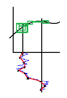
Visually this looks like:

Here the black curve represents $f(B_t)$, and the blue curve is Brownian motion, which oscillates and corresponding gives a value for $f(B_t)$. We also track the relative change of Brownian motion by $[B_{t_{n+1}}-B_{t_n}]$. This can generalize to $f(t,B_t)$ by introducing another dimension for time.
Quadratic variation arises when we consider the Ito isometry:
$$\mathbb{E} \left[ \left( \int_0^T X_t \, \mathrm{d} W_t \right)^2 \right] = \int_0^T \mathbb{E} \left[X_t^2\right] \, \mathrm{d} t$$
, where one squares the original integral and correspondingly gets terms involving $[B_{t_{n+1}}-B_{t_n}]^2$ in the numerical approximation and in the limit. Thus quadratic variation captures the relative drift of your stochastic process over an interval of time. The technical details are beyond the scope of this answer, but the basic need for quadratic variation arises because Brownian motion's total variation, $\sum_{i=0}^n|B_{t_{n+1}}-B_{t_n}|$ will almost surely diverge in the limit, whereas $\sum_{i=0}^n[B_{t_{n+1}}-B_{t_n}]^2$ will almost surely converge. The fact that quadratic variation converges allows one to make sense of Ito integrals (through an analog the Cauchy Schwartz inequality).

