PCA, dimensionality, and k-means results: reaction to duplicating of variables

Question

There are many excellent conversations on CV about the curse of dimensionality when applied to methods like k-means. The answer in the same post and other research (e.g., the paper titled "When Is ‘Nearest Neighbor’ Meaningful: A Converse Theorem and Implications") point that if the "intrinsic" domensionality of the data is lower then the curse does not apply.

However, I am coming from the angle of practical application, which seems to be not clearly answered.

Let's say we want to do k-means clustering in high dimensions. The data consists of $n$ rows and $d$ features. To make the conversation simpler, we can assume that the $d$ features are not independent and the intrinsic dimensionality of the data is actually $m$ such that $m<d$. To further simplify and for illustrative purposes, we can imagine two cases where the intrinsic dimensionality is the same but the correlation structure between the features is different:

1. All of the $m$ features are duplicated multiple times to create the data with $d$ features. For example, all the features are duplicated once and we get $d = 2m$.
2. Some of the $m$ features are duplicated to make up the $d$ features. For example, only the first feature is duplicated.

Now if PCA is run on this data then in both cases it will correctly say that the data is actually $m$ dimensional as 100% variance will be explained by the $m$ eigenvalues. Thus, one can conclude that the curse of dimensionality does not apply in either case and use all $d$ features to calculate distances between the points. However, the Euclidean distances in the two cases will be very different. Specifically, in the first case it will be the same as the $m$ dimensional data, while in the second case it will be biased.

Question: As we do not know the correlation structure of the data, should all analysis (e.g. k-means) be run on the $m$ PCA scores instead of the $d$ dimensional data?

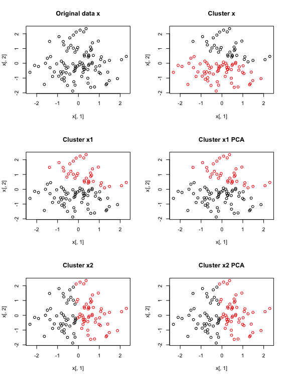
EDIT: I am adding some R code and the resulting plot to show that the k-means results actually differ. The data x is available here. The data x1 simply duplicates the features of x and the data x2 duplicates only the first feature of x. PCA on both x1 and x2 show that first two components retain ~100% of cumulative variance. So I expect that all the plots on the right hand column to show similar clustering.

set.seed(1)
x   <- matrix(rnorm(100*2), nrow=100)
x   <- scale(x, scale=FALSE)
x1  <- cbind(x, x) 
x2  <- cbind(x, x[,1]) 
k   <- kmeans(x,  2, iter.max=100, nstart=10)
k1  <- kmeans(x1, 2, iter.max=100, nstart=10)
k2  <- kmeans(x2, 2, iter.max=100, nstart=10)
p1  <- prcomp(x1)
p2  <- prcomp(x2)
kp1 <- kmeans(p1$x[,1:2], 2, iter.max=100, nstart=10)
kp2 <- kmeans(p2$x[,1:2], 2, iter.max=100, nstart=10)

par(mfrow=c(3,2))
plot(x[,1], x[,2], main="Original data x")
plot(x[,1], x[,2], col=k$cluster,   main="Cluster x")
plot(x[,1], x[,2], col=k1$cluster,  main="Cluster x1")
plot(x[,1], x[,2], col=kp1$cluster, main="Cluster x1 PCA")
plot(x[,1], x[,2], col=k2$cluster,  main="Cluster x2")
plot(x[,1], x[,2], col=kp2$cluster, main="Cluster x2 PCA")

Answer 1

If you duplicate any variable (of m variables) in multivariate data you do not expand the intrinsic (real) dimensionality which remains and is equal to the number of positive eigenvalues of the covariance matrix. By duplicating a variable you simply are adding one zero eigenvalue; you are also inflating positive m eigenvalues because you are adding variability to data by adding more values.

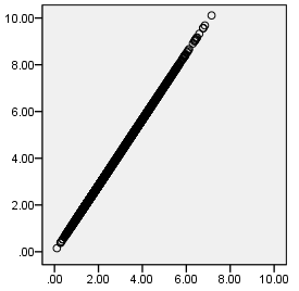
If you duplicated all the m variables equal number of times k you expanded the size of the data cloud (i.e. its dispersion about the centroid) without altering the shape of the data cloud: it still occupies the m subspace but it is bigger now: euclidean distances got longer, but proportionally - there was no bias introduced in the distance matrix (e.g., with single variable values, say, -1 and 1 the distance between the 2 points is 2; if you take that variable twice the distance is sqrt(8)=2.83). K-means done on original m and on new k*m variables will always yield same result if the same points are used as initial cluster centres. In fact, K-means works only within the real dimensionality where all data lie in, and so if initial centres do not depart from that subspace then centres being updated by the data will never leave that (sub)space. And because no bias with distances occured you arrive at the same clusters. If you prefer to do K-means on PCA scores of all the m componets extracted from the k*m variables, results will still not change (provided you use still same points for initial centers).

The following scatterplot shows distances within some data; X axis is distances in original data and Y axis is data with each variable duplicated. You can see that "nothing changed" except proportional increase.

If you duplicated only some of the m variables you are still in m intrinsic dimensionality, as before; however, the data cloud got expanded distortedly so euclidean distances increased not all proportionally. Some points (pairs) might have become relatively closer, some - relatively farther. That can influence the results of clustering, such as k-means. Irrespective whether you do the clustering based on all the many varables or on only the all m data's pr. components. You introduce more bias to distances if you duplicate just few variables many times.

For example, here is two variables:

  id       v1       v2
   1     1.00      .50
   2      .50      .50
   3    -1.00     -.50
   4     -.50      .00

Eigenvalues of the cov. matrix and Euclidean distances:

1.045900805 
 .016599195 

 .000000000    .500000000   2.236067978   1.581138830 
 .500000000    .000000000   1.802775638   1.118033989 
2.236067978   1.802775638    .000000000    .707106781 
1.581138830   1.118033989    .707106781    .000000000

Add 6 copies of v1 (but not v2) to the data. Now,

6.042387457 
 .020112543 
 .000000000 
 .000000000 
 .000000000 
 .000000000 
 .000000000 
 .000000000

 .000000000   1.322875656   5.385164807   4.000000000 
1.322875656    .000000000   4.092676386   2.692582404 
5.385164807   4.092676386    .000000000   1.414213562 
4.000000000   2.692582404   1.414213562    .000000000

Observe bias in distances. In old data, d(1,2)=.500 and d(3,4)=.707, so .707/.500 = 1.41. In new data, d(1,2)=1.323 and d(3,4)=1.414, so 1.414/1.323 = 1.07. Points 3-4 have become relatively closer to each other and are now almost as close as points 1-2, while before the duplicating they were farther apart than 1-2.

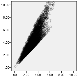
Duplicating some but not all of variables amounts to their (their importance) differential weighting. As it was explained, that of course tells upon distances differentially. The following scatterplot shows distances within some data; X axis is distances in original data and Y axis is data with some variables duplicated: some thrice, some twice (and some not duplicated). The shape is dispersed above the diagonal.

The majority of clustering algorithms will be affected by such altered distances. PCA scores (and clustering base on them) will be affected too, sure, despite that the intrinsic dimensionality doesn't change.

Answer 2

First, remember what the curse of dimensionality is. As the dimensionality of the data increases, if the data are uniformly distributed throughout the space, then the distribution of the distances between all points converges towards a single value. So to check this, we can look at the distribution of pairwise distances, as illustrated in @hdx1011's answer. If all the distances are approximately the same, that is a problem for clustering algorithms like k-means, because it is trying to partition the data into sets of 'closer together' distinct from the other subsets of the data which are relatively 'further away'. But if they are all the same distance apart, this is logically impossible.

One of the points I was trying to make in my answer there, was that data are often not uniformly distributed in the space such that the "effective dimensionality" is not the same as the "literal dimensionality" (note that these are not formal mathematical terms). In the comments, @ttnphns explains that "intrinsic dimensionality m is the number of positive eigenvalues", which is the rank of the matrix. This is true, and your example of duplicating variables will yield a matrix whose rank is less than the number of resulting variables, but this isn't quite what I was getting at. You can very well have a matrix of full rank in which the curse of dimensionality does not apply because the effective dimensionality is much lower.

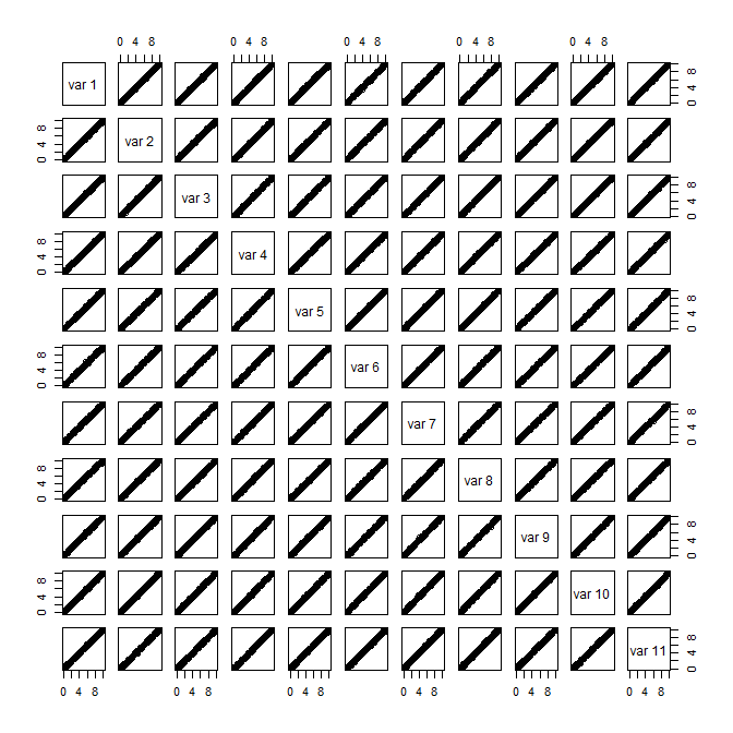
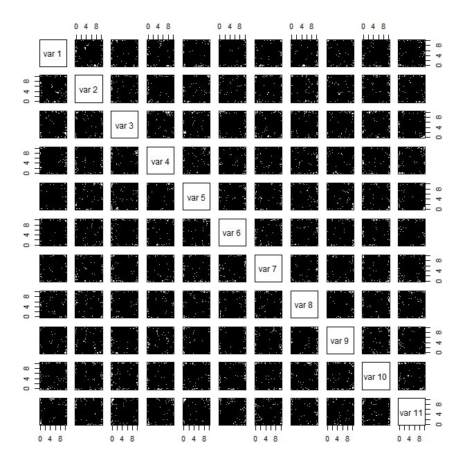
Below is an example, coded in R. I generate two datasets; the first has eleven variables, each of which is a manifestation of a single latent variable, with a small amount of noise, whereas the second is a set of roughly orthogonal uniform variables. Both matrices have rank $11$ (with eleven positive eigenvalues), but the first is essentially one-dimensional. The scatterplot matrices make this obvious.

set.seed(9381)  # this makes the example exactly reproducible
lat.var   = runif(500, min=0, max=10)                   # a single latent variable
C.dat.mat = matrix(lat.var+rnorm(5500, mean=0, sd=.1),  # 10 manifest vars w/ noise
                 nrow=500, ncol=11, byrow=FALSE)
qr(C.dat.mat)$rank  # [1] 11
round(eigen(cor(C.dat.mat))$values, digits=3)
# [1] 10.988 0.001 0.001 0.001 0.001 0.001 0.001 0.001 0.001 0.001 0.001

set.seed(9381)
U.dat.mat = matrix(runif(5500, min=0, max=10),          # 10 orthogonal, unif vars
                   nrow=500, ncol=11, byrow=FALSE)
qr(U.dat.mat)$rank  # [1] 11
round(eigen(cor(U.dat.mat))$values, digits=3)
#  [1] 1.266 1.188 1.121 1.041 1.031 1.011 0.938 0.904 0.874 0.845 0.781

windows()
  pairs(C.dat.mat)
windows()
  pairs(U.dat.mat)

If we examine all pairwise distances, we see that the distances of the orthogonal, uniform variables are becoming compressed into a narrower range of similar values. Specifically, for the correlated data, the middle $50\%$ are within $(4.5, 16.6)$, but for the uniform data, the middle $50\%$ are only in $(11.7, 15)$. The curse of dimensionality just isn't 'biting' for the former set, despite the fact that there are eleven variables and the matrix is full rank.

dist.vector = function(dat){    # this function computes all pairwise distances
  dists = as.matrix(dist(dat))
  return(as.vector(dists[upper.tri(dists)]))
}
L.dists = dist.vector(lat.var)    # for only the latent variable
C.dists = dist.vector(dat.mat)    # for the correlated dataset
U.dists = dist.vector(U.dat.mat)  # for the orthogonal uniform dataset

summary(lat.var)  # hinge points of the latent variable
#    Min. 1st Qu.  Median    Mean 3rd Qu.    Max. 
# 0.02661 2.54400 4.93200 5.00200 7.39100 9.99900 
summary(L.dists)  # hinge points of the pairwise distances of the latent variable
#     Min.  1st Qu.   Median     Mean  3rd Qu.     Max. 
# 0.000033 1.346000 2.931000 3.337000 5.013000 9.973000 
summary(C.dists)  # ... of the correlated matrix
#    Min. 1st Qu.  Median    Mean 3rd Qu.    Max. 
#  0.1913  4.4820  9.7350 11.1000 16.6300 33.1000 
summary(U.dists)  # ... of the orthogonal, uniform matrix
#    Min. 1st Qu.  Median    Mean 3rd Qu.    Max. 
#   3.126  11.660  13.370  13.330  15.030  22.970 

---

As a footnote, you are generating matrices that are not full rank. To understand the effect of that on a principal components analysis, you may want to read this excellent CV thread: Should one remove highly correlated variables before doing PCA?

Answer 3

I couldn't perfectly make sense of the question, but here is an answer: when you do PCA on a dataset, you learn a new basis (say $t$ dimensional, $t<d$), where the variation in the data is represented more compactly. The first basis vector is the direction, where the most variation was in the original $d$ dimensional trivial basis etc... One thing to notice is that this basis is an orthonormal basis.

Euclidean norm, or Frobenius norm for matrices are invariant to basis changes with orthonormal bases. This means, the basis change will actually not change your landscape for the k-means clustering. Hence there is no difference in doing the clustering in either of the domains.

Answer 4

If you duplicate every attribute y times, the resulting squared Euclidean distances will be exactly y times larger.

But then k-means will still assign every point to the exact same "nearest" center. So the results are entirely unaffected.

Instead of duplicating them, also add a small random error each.