Introducing seasonality to an ARIMA model in R

Question

Using the forecast package, I am constructing a dynamic regression / ARIMA model to use X to predict Y (data below). Here is my model:

fit <-auto.arima(y,xreg=x,seasonal=c(0,1,1)[4])
summary(fit)

Question - I'm not sure I am using the seasonal portion of code correctly:

seasonal=c(0,1,1)[4]

I see no difference in the forecasts using the above seasonality code and not including the seasonality code at all.

Question: How do I specify seasonality in this instance? Is there a way the arima code can automatically detect correct seasonality and specify it in code?

Data:

qtrs     y         x
1Q14    41.7    16963482
2Q14    26      8857757
3Q14    22.4    6308120
4Q14    17.6    4872037
1Q15    47.7    20304915
2Q15    30.7    8800350
3Q15    25.6    8065914
4Q15    17.4    8.41E+06
1Q16    59.4    39076150
2Q16    35.6    23348752
3Q16    33.5    26721456
4Q16    23.9    17934787
1Q17    81.7    65821538
2Q17    44.8    35845803
3Q17    42.1    34753415
4Q17    28.5    21449909
1Q18    90      84207978

or also

> dput(y)
c(41.7, 26, 22.4, 17.6, 47.7, 30.7, 25.6, 17.4, 59.4, 35.6, 33.5, 
23.9, 81.7, 44.8, 42.1)
dput(x)
c(16963482, 8857757, 6308120, 4872037, 20304915, 8800350, 8065914, 
8410000, 39076150, 23348752, 26721456, 17934787, 65821538, 35845803, 
34753415)

When I use:

   fit <-auto.arima(y,xreg=x,seasonal=True)

it returns:

  summary(fit)
  Series: y 
  Regression with ARIMA(0,1,0) errors 

 Coefficients:
      x
  0e+00
  s.e.  3e-04

  sigma^2 estimated as 24.53:  log likelihood=-41.75
  AIC=87.49   AICc=88.58   BIC=88.77

  Training set error measures:
                ME     RMSE      MAE      MPE     MAPE      MASE       ACF1
  Training set -1.521487 4.611119 3.659424 -7.34176 12.28209 0.1975017 -0.2619158

But when I use the below, it returns the same as above. fit <-auto.arima(y,xreg=x,seasonal=c(0,1,1)[4])

Why is there no seasonal variables in this model when there clearly is seasonality? Why no difference in the two models (seasonality specified and not specified)?

Answer 1

The seasonal parameter expects a simple Boolean input (see ?auto.arima). What you are providing is c(0,1,1)[4], which happens to be a well-formed R expression, namely the fourth entry in the vector c(0,1,1) of length three, or

c(0,1,1)[4]
# NA

And this NA is then coerced to a Boolean value, namely

isTRUE(NA)
# FALSE

So what you did was an elaborate way of specifying a non-seasonal model. Try seasonal=TRUE instead.

(And don't be surprised if the automatic model selection decides to use a non-seasonal model, anyway. If you want to force seasonality, this may be helpful: Seasonality not taken account of in auto.arima().)

---

EDIT: with the data you posted, the first thing to notice is that x and y are vectors, not time series objects with an associated seasonal frequency. As above, auto.arima does not derive the seasonal period from the seasonal parameter (which is supposed to be, and will be coerced to, a simple Boolean), but from the frequency of the focal time series. So the first thing to do is to identify your quarterly data as such:

y <- ts(c(41.7, 26, 22.4, 17.6, 47.7, 30.7, 25.6, 17.4, 59.4, 35.6, 33.5, 
  23.9, 81.7, 44.8, 42.1), frequency=4)
x <- ts(c(16963482, 8857757, 6308120, 4872037, 20304915, 8800350, 8065914, 
  8410000, 39076150, 23348752, 26721456, 17934787, 65821538, 35845803, 
  34753415),frequency=4)

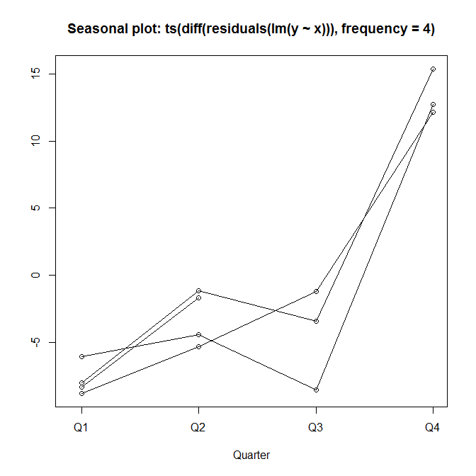
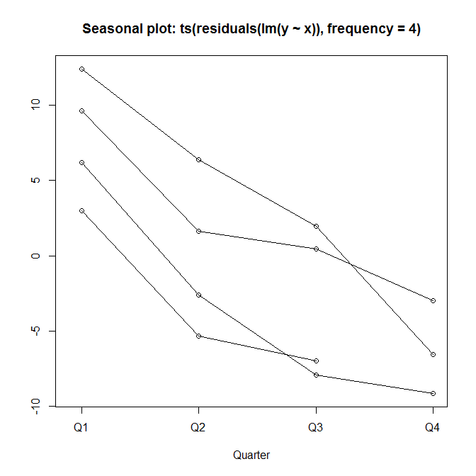
Next, even if your y is seasonal, this does not necessarily matter. auto.arima() with an xreg parameter fits a regression with ARIMA errors (not ARIMAX), so what matters is the seasonality of the residuals of this regression of y on x. Fortunately, these residuals are also clearly seasonal, as are their first differences (note how we again need to convert the residuals to ts objects):

library(forecast)
seasonplot(ts(residuals(lm(y~x)),frequency=4))
seasonplot(ts(diff(residuals(lm(y~x))),frequency=4))

Interestingly enough, auto.arima() fits a non-seasonal model, as you noticed, even if we don't specify seasonal=FALSE. Then again, if we call auto.arima() on the residuals from the regression y~x, we get a seasonal model, and so do we if we run auto.arima(y,xreg=x,D=1) with enforced seasonality as per this thread - but the seasonal models are different.

> auto.arima(y,xreg=x)
Series: y 
Regression with ARIMA(0,1,0) errors 

Coefficients:
       xreg
      0e+00
s.e.  3e-04

sigma^2 estimated as 24.53:  log likelihood=-41.75
AIC=87.49   AICc=88.58   BIC=88.77

> auto.arima(ts(residuals(lm(y~x)),frequency=4))
Series: ts(residuals(lm(y ~ x)), frequency = 4) 
ARIMA(0,1,0)(1,0,0)[4] 

Coefficients:
        sar1
      0.9074
s.e.  0.0694

sigma^2 estimated as 12.65:  log likelihood=-40.58
AIC=85.16   AICc=86.25   BIC=86.44

> auto.arima(y,xreg=x,D=1)
Series: y 
Regression with ARIMA(0,0,0)(0,1,0)[4] errors 

Coefficients:
       xreg
      0e+00
s.e.  3e-04

sigma^2 estimated as 12.29:  log likelihood=-28.88
AIC=61.76   AICc=63.26   BIC=62.56

Overall, it looks like there is something undocumented going on here - auto.arima() may by default not use seasonal models if there is an xreg present. You may want to ping the author Rob Hyndman about this (best to point him to this thread, he may chime in). Similarly, that the last two calls resulted in different ARIMA models may be due to internals of auto.arima().

It looks like your best bet may be to run the regression outside auto.arima() and then subject the residuals to ARIMA modeling, as I did here. Alternatively, if you can identify whether your residual series is seasonal or not, you can enforce seasonality using D as above.

Answer 2

Are you sure that's the best seasonal set-up? What I mean is that if you use auto.arima to find the "best" model, you might as use it to find the best seasonal configuration as well? If you leave it out, auto.arima will test automatically for seasonality