Measuring skewness of abundance over time

Question

I have measurements of flower counts thru time for a bunch of species and locations. I'm interested in whether they are more or less "normally" distributed, with a peak in the middle and symmetric, or skewed to the left or right in time. It seems like I would be able to do this with various skewness tests or fitting different distributions, but since these are not histograms but timeseries I feel like that would be incorrect.

Here is some example data of a skewed timeseries and one that is fairly symmetric.

skewed_counts = c(2,9,17,32,40,32,12,11,9,2,2,5,5,3,4,2,1,1,2,2,1,1,1,1)
skewed_time = c(202,204,206,208,210,212,215,217,219,221,222,224,226,228,230,232,236,238,240,242,244,246,248,250)

symmetric_counts = c(1,8,8,26,42,48,66,52,63,20,18,27,6,3)
symmetric_time = c(188,190,192,194,196,198,200,202,204,206,208,210,212,214)

Answer 1

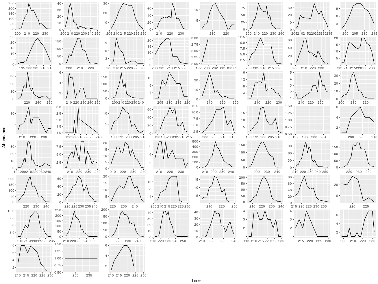
Actually, you can interpret your data as a histogram if you consider the time of each individual observation of a flower as a random variable. Time histograms are used all the time, for example, in neuroscience (See, e.g., "A Method for Selecting the Bin Size of a Time Histogram").

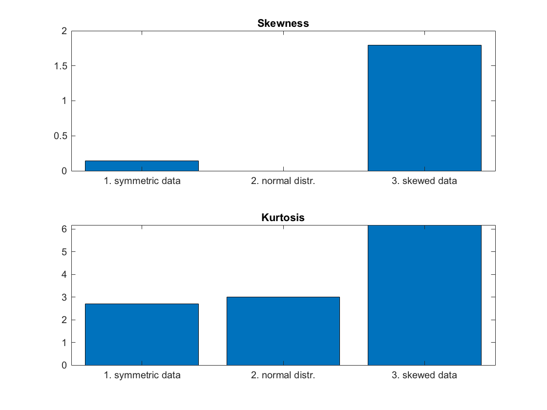
So it's fine to test for normality of your data (using any one of several tests), but it sounds like you are more interested in checking for symmetry and a small tail, properties that are not unique to the normal distribution. You can use skewness and kurtosis to do this.

You seem to be familiar with skewness, which measures symmetry. However, as you have intuited, low skewness is not a sufficient condition for the shape you are looking for because, e.g., the data in row 2, column 8 is symmetric but bimodal. You can use kurtosis to quantify this deviation from a central peak and compare it to the normal distribution, which has a kurtosis value of 3.

Here is some Matlab code to compute this for your example data:

skewTime = [202,204,206,208,210,212,215,217,219,221,222,224,226,228,230,232,236,238,240,242,244,246,248,250];
skewCount = [2,9,17,32,40,32,12,11,9,2,2,5,5,3,4,2,1,1,2,2,1,1,1,1];
symCount = [1,8,8,26,42,48,66,52,63,20,18,27,6,3];
symTime = [188,190,192,194,196,198,200,202,204,206,208,210,212,214];

% Turn the data into sets of individual time-valued observations
Nskew = length(skewCount);
skewData = [];
for i = 1:Nskew
    skewData = [skewData repmat(skewTime(i),[1 skewCount(i)])];
end

Nsym = length(symCount);
symData = [];
for i = 1:Nsym
    symData = [symData repmat(symTime(i),[1 symCount(i)])];
end

% Calculate kurtosis
Kskew = kurtosis(skewData);
Ksym = kurtosis(symData);
Knorm = 3;
% Calculate skewness
Sskew = skewness(skewData);
Ssym = skewness(symData);
Snorm = 0;

c = categorical({'1. symmetric data','2. normal distr.','3. skewed data'});

figure
subplot(211)
bar(c,[Ssym,Snorm,Sskew]), title('Skewness')
subplot(212)
bar(c,[Ksym,Knorm,Kskew]), title('Kurtosis')