Simple explanation of dynamic linear models

Question

I'm looking for a really simple explanation of what a dynamic linear model is as I need to explain this to a non-technical audience. I have looked around for examples but they are very maths heavy.

I found this explanation below from the dlmodeler vignette:

http://www2.uaem.mx/r-mirror/web/packages/dlmodeler/dlmodeler.pdf (see pages 2 and 3)

There are still aspects of it that I think the audience won't follow so am looking for someone to provide a very basic explanation or example that illustrates broadly how dlms work (would be great if the examples were in R).

Thanks

---

Introduction

Generalized Dynamic Linear Models are a powerful approach to time-series modelling, analysis and forecasting. This framework is closely related to the families of regression models, ARIMA models, exponential smoothing, and structural time-series (also known as unobserved component models, UCM).

The origin of DLM time-series analysis has its roots in the world of engineering. In order to control dynamic physical systems, unknown quantities such as velocity and position (the state of the system) need to be estimated from noisy measurements such as readings from various sensors (the observations). The state of the system evolves from one state (e.g. position and speed at time t) to another (position and speed at time t+1) according to a known transition equation, possibly including random perturbations and intervention effects. The observations are derived from the state values by a an observation equation (e.g. observation at time t = position + noise), also possibly including random disturbances and intervention effects.

The challenge is to obtain the best estimate of the unknown state considering the set of available observations at a given point in time. Due to the presence of noise disturbances, it is generally not possible to simply use the observations directly because they lead to estimators which are too erratic. During the 1960s, the Kalman filtering and smoothing algorithm was developed and popularized to efficiently and optimally solve this estimation problem. The technique is based on an iterative procedure in which state values are successively predicted given the knowledge of the past observations, and then updated upon the reception of the next observation. Because of the predict-and-update nature of Kalman filtering, it can also be interpreted under a Bayesian perspective.

Dynamic linear models

The theory developed for the control of dynamic systems has a direct application to the general analysis of time-series. By having a good estimate of the current state and dynamics of the system, it is possible to derive assumptions about their evolution and subsequent values; and therefore to obtain a forecast for the future observations.

Dynamic Linear Models are a special case of general state-space models where the state and the observation equations are linear, and the distributions follow a normal law. They are also referred to as gaussian linear state-space models. Generalized DLMs relax the assumption of normality by allowing the distribution to be any of the exponential family of functions (which includes the Bernoulli, binomial and Poisson distributions, useful in particular for count data).

There are two constitutive operations for dynamic linear models: filtering and smoothing. In a few words, filtering is the operation consisting in estimating the state values at time t, using only observations up to (and including) t-1. On the contrary, smoothing is the operation which aims at estimating the state values using the whole set of observations.

Answer 1

I also have to speak regularly to people who do not have a technical background, and here is how I would approach it: First, unless your audience knows about the normal distribution, I would not even mention DLM, I would just talk about state space models. I would still give them a DLM set of equations as an example (linear is easy to understand), but I have found that it is very very easy to talk to people without a technical background about the "observed" and the "state" equation.

I would then illustrate it with a simple example (that I take from the "Dynamic Linear Models with R" book by Petris, Petrone and Campagnoli 2009). Here is what I would say (roughly) to an audience to explain them what the main point of DLM is:

Speaker: "Suppose you are interested in measuring the level of the river Nile, e.g. because you want to have an idea during which period of the year certain ships (with different sizes) can sail through it or because you are just interested in seeing how the long term water level changes throughout time.

Every year, you go to a certain spot along the river and you take a measurement. Now, it could happen that on that day it was raining, or even it was raining throughout the whole month, or that you did not measure precisely because your equipment was not too good, right? So the main premise is that you measure the water level with an additional, not controllable and random imprecision. To make things a bit more specific:

$Observed Nile Water Level_t$ = $True Nile Water Level_t + Measurement Error_t$

We see that every year that we measure the water level, it is a function of some true level and a measurement error that is always there (but has a random nature) and cannot be avoided ( Here I find the example with the rain on the day that you measure very good to illustrate where the error term can come from)

That's all well and good, but it also makes sense to assume that the true Nile water level changes throughout time, right? Maybe people build dams and stop some of the inflow from the smaller rivers or something like that.

Well, then it makes sense to also incorporate the following equation right?:

$True Nile Water Level_t $ = $True Nile Water Level_{t-1} + Additive Error_t$

The true, unobserved level of today depends on the level from last year and some other part that we put in, which is random, and expresses our inability to estimate things perfectly."

This is roughly the way that I have explained it to audience that is not technical (but they had finance background so I was using "underlying state of the economy" as an example).

This is also the random walk + noise model and it is the simplest DLM I can think of (if they don't know what a regression is, forget about talking to them about random slopes and so on). Obviously you can still scale the example up, if you think that they have at least some exposure to statistical models and discuss random slope etc.

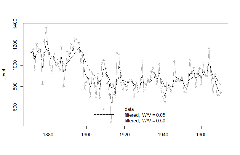
Here is the code for the filtered values of the Nile Rirver Level (I took it from the book, you can find it here) and if you cannot find the book, you can access the corresponding article for free from JStatSoft here

###
plot(Nile, type='o', col = c("darkgrey"),
     xlab = "", ylab = "Level")
mod1 <- dlmModPoly(order = 1, dV = 15100, dW = 755)
NileFilt1 <- dlmFilter(Nile, mod1)
lines(dropFirst(NileFilt1$m), lty = "longdash")
mod2 <- dlmModPoly(order = 1, dV = 15100, dW = 7550)
NileFilt2 <- dlmFilter(Nile, mod2)
lines(dropFirst(NileFilt2$m), lty = "dotdash")
leg <- c("data", paste("filtered,  W/V =",
                       format(c(W(mod1) / V(mod1),
                                W(mod2) / V(mod2)))))
legend("bottomright", legend = leg,
       col=c("darkgrey", "black", "black"),
       lty = c("solid", "longdash", "dotdash"),
       pch = c(1, NA, NA), bty = "n")

The example shows the fit with different signal to noise ratios - the higher the signal to noise, the better the "fit". I think it is instructive to see that but you can skip it and just show the fitted line.

If your audience can take it, talk to them about forecasting, filtering and smoothing with the Kalman Filter (but if they are not technical, skip it). And obviously you can fit other models to that data.

Hope this helps, let us know what you think and what you presented to them at the end!

EDIT: I actually just now saw that this thread was necroed from 4 months ago...even if the OP is way past needing this, I hope it would be useful to someone in the future.

Answer 2

I recommend that you go through a few examples. The most common question is "what does the state variable represent?" The answer to that depends on the model, but most DLMs can be thought of as a regression with a time-varying coefficient. In this context, those time-varying coefficients are your states usually.

If you regress on an intercept, they sometimes call that model a local level model. If you regress on past values of the process, sometimes they call that a time-varying autogression. You can also regress on harmonics or polynomials in time. All of these have in common that they're basically regression, but you put dynamics on the coefficients.

Answer 3

Best I can do is a tad lengthy but perhaps easier to follow (1st try):

So for a (static) linear regression, the usual format is y = mx +b, like the equation of a line (b is a constant, m is the slope, x are your predictors, y is your response).

The magic of regression is that it amps up this equation to the matrix level (so now we have a line in an n-dimensional space and not the usual 2-dimensional line residing in the x-y plane like above), so now more like Y= MX + b where Y and X (and M) are matrices, and regression determines our M and our b through a bunch of matrix algebra, likelihood estimation or etc. We can do this because we know the data exists in multiple observations like Y(i) = MX(i)+b for all values of i, up to our number of observations.

But for time series, sequential data, this i is really a time step t, so now more like Y(t) = MX(t) + b, BUT now we can do a trick. Instead of assuming M is a matrix of static slopes to be determined by the data, what if we assume M is not a set of fixed values across all the observations over time, but instead a changing, dynamic, update-able set of slopes that are related to the prior time step, t-1, for all steps of t?

This would stand to reason because in a time series, the last value of y(t-1) is related to the next value of y(t) generally (this is auto-regressive and can be tested for). There is no reason to believe M doesn't change over time too so why not check it out. To do this we insert a few more 'internal parameters' in our regression set up that allow for changing conditions at different (but sequential) t to take advantage of this y(t) to y(t-1) relationship.

Dynamic regression allows our M, our slopes (i.e. our regression parameters i.e. the effect sizes of our predictors) to change over time and may give us better abilities and insight as to what is going on (rather than treating every parameter in M as 'static' at all t, but the parameters that evolve and change across the flow of t) -- - -

Sometimes it helps, other times other 'non-stationary' analysis helps (like ARIMA and straight auto-regressive AR(1), etc) -- - -