Completely different results from lme() and lmer()

Question

I've been playing around with both nlme::lme and lme4::lmer. I fitted a simple random intercepts model using lme() and lmer(). As you can see below, I got completely different results from lmer() and lme(). Even signs of coefficients are different! Am I doing something wrong? I also fitted an empty model with the two packages. In this case, the results were practically the same (results not shown). Would you educate me to understand this issue? Unless I made a mistake, I think there is something wrong with the lme4 package.

     multi <- structure(list(x = c(4.9, 4.84, 4.91, 5, 4.95, 3.94, 3.88, 3.95, 
4.04, 3.99, 2.97, 2.92, 2.99, 3.08, 3.03, 2.01, 1.96, 2.03, 2.12, 
2.07, 1.05, 1, 1.07, 1.16, 1.11), y = c(3.2, 3.21, 3.256, 3.25, 
3.256, 3.386, 3.396, 3.442, 3.436, 3.442, 3.572, 3.582, 3.628, 
3.622, 3.628, 3.758, 3.768, 3.814, 3.808, 3.814, 3.944, 3.954, 
4, 3.994, 4), pid = 1:25, gid = c(1L, 1L, 1L, 1L, 1L, 2L, 2L, 
2L, 2L, 2L, 3L, 3L, 3L, 3L, 3L, 4L, 4L, 4L, 4L, 4L, 5L, 5L, 5L, 
5L, 5L)), class = "data.frame", row.names = c(NA, -25L))

#lme
> lme(y~x, random=~1|gid,data=multi,method="REML")
Linear mixed-effects model fit by REML
  Data: multi 
  Log-restricted-likelihood: 41.76745
  Fixed: y ~ x 
(Intercept)           x 
  4.1846756  -0.1928357 

#lmer

 lmer(y~x+(1|(gid)), data=multi, REML=T)
    Linear mixed model fit by REML ['lmerMod']
    Formula: y ~ x + (1 | (gid))
       Data: multi
    REML criterion at convergence: -78.4862
    Random effects:
     Groups   Name        Std.Dev.
     (gid)    (Intercept) 0.70325 
     Residual             0.02031 
    Number of obs: 25, groups:  (gid), 5
    Fixed Effects:
    (Intercept)            x  
         2.8152       0.2638 

Answer 1

As it was noted in this answer, and also mentioned in one of the comments, the problem seems to be a local maximum. To see this more clearly I have written below a simple code to calculate the negative log-likelihood of this model and do the optimization using optim(). Starting with different initial values leads to the two different solutions:

# data
multi <- structure(list(x = c(4.9, 4.84, 4.91, 5, 4.95, 3.94, 3.88, 3.95, 
                              4.04, 3.99, 2.97, 2.92, 2.99, 3.08, 3.03, 2.01, 1.96, 2.03, 2.12, 
                              2.07, 1.05, 1, 1.07, 1.16, 1.11), 
                        y = c(3.2, 3.21, 3.256, 3.25, 
                              3.256, 3.386, 3.396, 3.442, 3.436, 3.442, 3.572, 3.582, 3.628, 
                              3.622, 3.628, 3.758, 3.768, 3.814, 3.808, 3.814, 3.944, 3.954, 
                              4, 3.994, 4), 
                        pid = 1:25, 
                        gid = c(1L, 1L, 1L, 1L, 1L, 2L, 2L, 
                                2L, 2L, 2L, 3L, 3L, 3L, 3L, 3L, 4L, 4L, 4L, 4L, 4L, 5L, 5L, 5L, 
                                5L, 5L)), class = "data.frame", row.names = c(NA, -25L))

# function to calculate the negative log-likelihood of the random intercepts model
library("mvtnorm")
logLik <- function (thetas, y, X, id) {
    ncX <- ncol(X)
    betas <- thetas[seq_len(ncX)]
    sigma_b <- exp(thetas[ncX + 1])
    sigma <- exp(thetas[ncX + 2])
    eta <- c(X %*% betas)
    unq_id <- unique(id)
    n <- length(unq_id)
    lL <- numeric(n)
    for (i in seq_len(n)) {
        id_i <- id == unq_id[i]
        n_i <- sum(id_i)
        V_i <- matrix(sigma_b^2, n_i, n_i)
        diag(V_i) <- diag(V_i) + sigma^2
        lL[i] <- dmvnorm(y[id_i], mean = eta[id_i], sigma = V_i, log = TRUE)
    }
    - sum(lL, na.rm = TRUE)
}

# optimization using as initial values 0 for the fixed effects, 
# and 1 for the variance components 
opt <- optim(rep(0, 4), logLik, method = "BFGS", 
             y = multi$y, X = cbind(1, multi$x), id = multi$gid)

opt$par[1:2] # fixed effects
#> [1] 2.855872 0.250341
exp(opt$par[3]) # sd random intercepts
#> [1] 0.6029724
exp(opt$par[4]) # sd error terms
#> [1] 0.01997889

# optimization using as initial values 4 & -0.2 for the fixed effects, 
# and 0.0003 and 0.034 for the variance components 
opt2 <- optim(c(4, -0.2, -8, -3.4), logLik, method = "BFGS", 
              y = multi$y, X = cbind(1, multi$x), id = multi$gid)

opt2$par[1:2] # fixed effects
#> [1]  4.1846965 -0.1928397
exp(opt2$par[3]) # sd random intercepts
#> [1] 0.000270746
exp(opt2$par[4]) # sd error terms
#> [1] 0.03239167

Answer 2

I agree with @DimitrisRizopoulos's answer, and have a few more points to make.

• I will start by saying that I am unhappy that lmer doesn't find the best answer - even though I suspect this situation is probably limited to small, unusual (see below) data sets. One of the reasons that lme may do better is that it fits on the log-standard-deviation scale, which may make the minimum near zero "broader".
• You can get lmer to replicate the lme results by setting an explicit, lower starting value for the scaled standard deviation (start=...); based on the explorations below, start=8 or any lower value should work OK. For what it's worth, this will lead to an estimated random effects variance of 0 (and a "singular fit" message, and an answer that's equivalent to leaving out the random effects component entirely and using lm() ...)
• In this particular case using the "nloptwrap" optimizer doesn't help; in fact all of the optimizers that lmer can use, starting from the default starting values ($\theta$ (scaled standard deviation) = 1.0), find the higher local minimum away from zero.
• here is code equivalent to the approach lmer uses to find the starting value by default, when only intercept-valued random effects are present (see here):

v0 <- with(multi,var(ave(y,gid)))  ## variance among group values  
v.e <- var(multi$y)-v0             ## residual var ~ total var - group variance
sqrt(v0/v.e)                       ## convert to scaled standard deviation

This leads to a starting value of $\theta=10.8$.

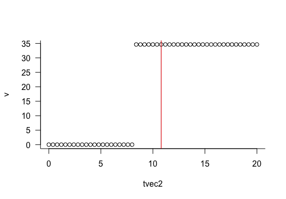
• We can see systematically how different starting values give different results:

m0 <- lmer(y~x+(1|(gid)), data=multi, REML=TRUE)
tvec2 <- seq(0,20,length=51)
ff <- function(t0) getME(update(m0,start=t0),"theta")
v <- sapply(tvec2,ff)
plot(tvec2,v)
abline(v=10.8,col="red")

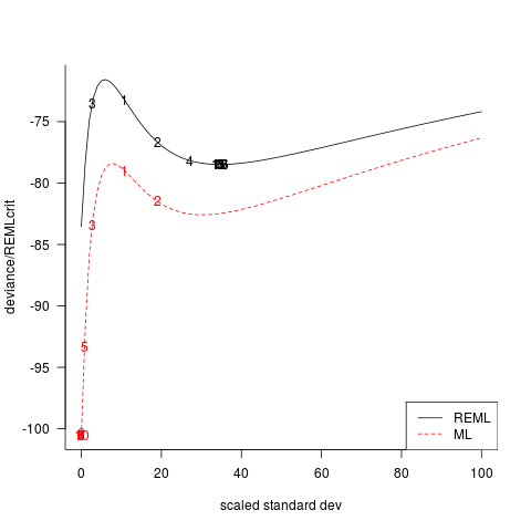
• We can also explicitly visualize the (negative log-)likelihood surface:

## helper function to capture fitting trajectory
cfun  <- function(...) {
    cc <- capture.output(x <- do.call(lmer,c(list(...),list(verbose=100))))
    gfun <- function(x,s) {
        as.numeric(gsub(s,"",grep(s,x,value=TRUE)))
    }
    it <- gfun(cc,"iteration: +")
    xval <- gfun(cc,"\tx = ")
    fval <- gfun(cc,"\tf\\(x\\) = +")
    attr(x,"optvals") <- data.frame(it,xval,fval)
    return(x)
}

c0 <- cfun(y~x+(1|(gid)), data=multi, REML=TRUE)
c1 <- cfun(y~x+(1|(gid)), data=multi, REML=FALSE)

f <- as.function(m0)
tvec <- seq(0,100,length=101)
dvec <- sapply(tvec,f)
m3 <- update(m0,REML=FALSE)
f2 <- as.function(m3)
dvec2 <- sapply(tvec,f2)
par(las=1,bty="l")
matplot(tvec,cbind(dvec,dvec2),type="l",
        ylab="deviance/REMLcrit",
        xlab="scaled standard dev")
with(attr(c0,"optvals"),text(xval,fval,it))
with(attr(c1,"optvals"),text(xval,fval,it,col=2))
legend("bottomright",c("REML","ML"),
       col=1:2,lty=1:2)

The numbers show the sequence of values tried. We can see that it is only the slightly different shape of the ML curve that tips the optimizer toward the boundary fit rather than the interior fit.

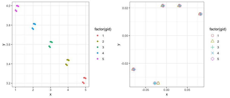
• Are these data artificial? The left plot below shows the data by group; the right plot shows the values with their group means subtracted. There is almost no variation among the 5 values within each group ...

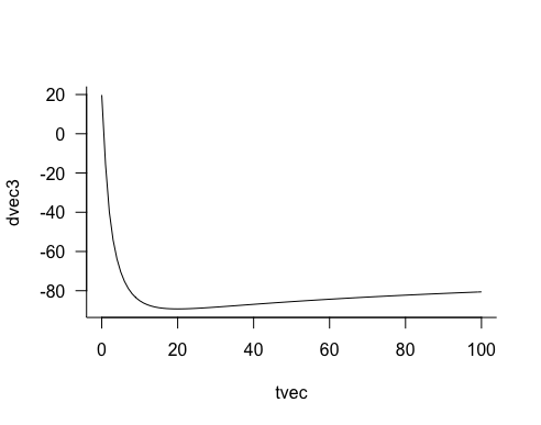
• If we simulate data with the same properties (starting from the estimated coefficients), but where the variation is actually Gaussian, we don't get the same kind of multimodal surface at all:

multi_sim <- transform(multi,y=simulate(m0,seed=101)[[1]])
f3 <- as.function(update(m0,data=multi_sim))
dvec3 <- sapply(tvec,f3)
plot(tvec,dvec3,type="l")