I'm working on a case study from this MIT course. I'm practicing classification problems.
Here is the code for my model. (The dataset can be accessed from the link. I can add it to this post)
    idx <- sample(seq(1, 3), size = nrow(Book), replace = TRUE,
                  prob = c(.45, .35, .2))
    train <- Book[idx == 1,]
    val <- Book[idx == 2,]
    test <- Book[idx == 3,]

    glm.fit1 <- glm(Florence ~., family = binomial,
                    data = train)
    summary(glm.fit1)
    glm.probs1 <- predict(glm.fit1, test, type='response')
    glm.pred1 <- rep("0",nrow(test))
    glm.pred1[glm.probs1 >.5] <- "1"
This is the confusion matrix
    > table(glm.pred1, test$Florence)

    glm.pred1   0   1
            0 787  73
            1   0   1
I have tried a few subsets of predictors and they have performed poorly.
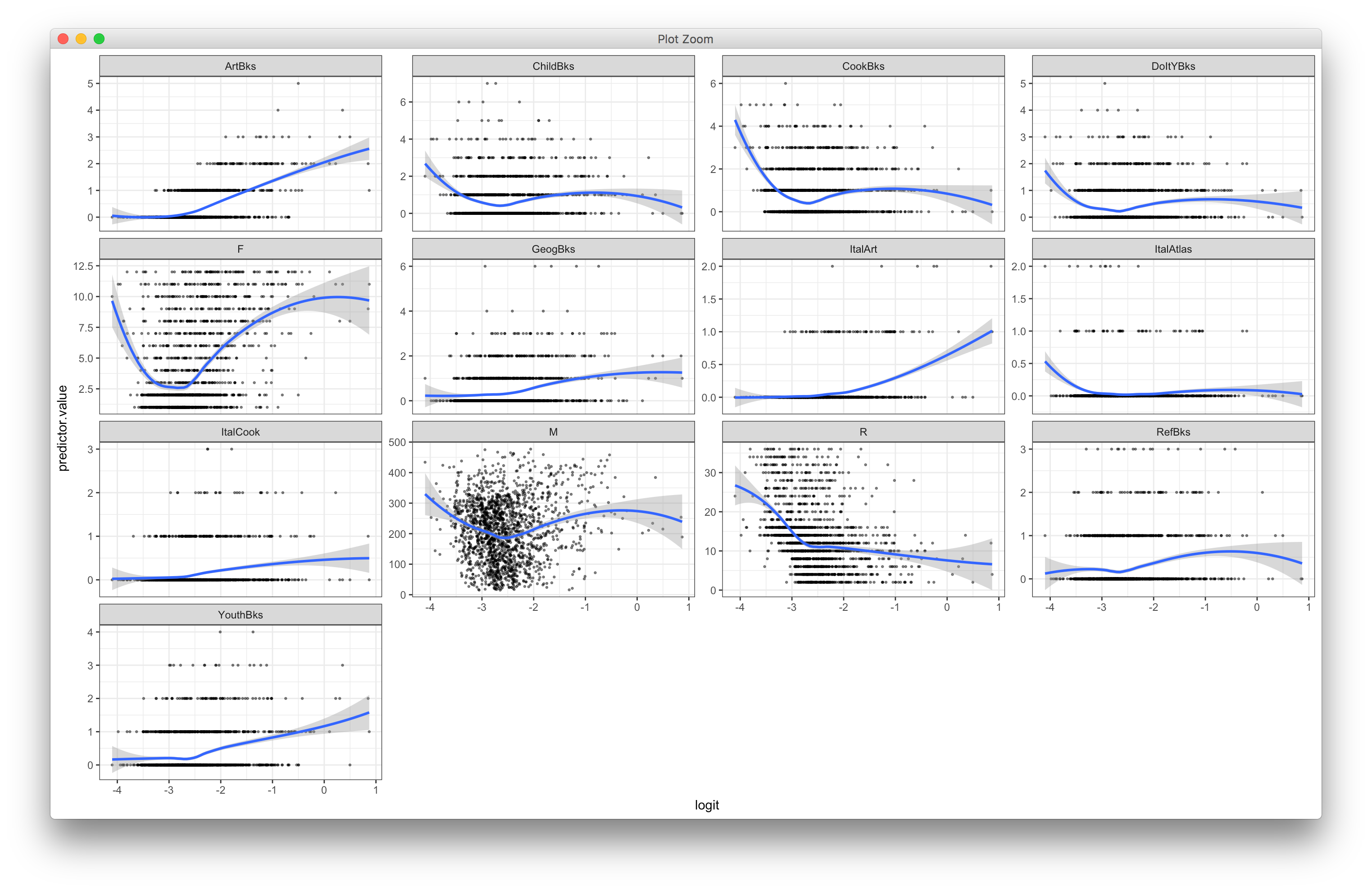
I checked for linearity relationship between the logit of the outcome and each predictor variables.
    # Select only numeric predictors
    num.train <-  num_vars(train)
    # Bind the logit and tidying the data for plot
    num.train <- num.train %>%
      mutate(logit = log(probabilities/(1-probabilities))) %>%
      gather(key = "predictors", value = "predictor.value",
             -logit)

    ggplot(num.train, aes(logit, predictor.value)) +
      geom_point(size = 0.5, alpha = 0.5) +
      geom_smooth(method = "loess") +
      theme_bw() +
      facet_wrap(~predictors, scales = "free_y")
The correlation between my predictors and response are largely weak and the relationships appear to be mostly non-linear. How do you adjust them to fit the assumptions for logistic regression?

