What are the assumptions of a Gamma GLM or GLMM for hypothesis testing?

Question

What are the assumptions when doing hypothesis testing using a Gamma GLM or GLMM? Are the residuals suppose to be normally distributed and is heteroscedasticity a concern like the Gaussian (normal) distribution? Do you test the assumptions in the same fashion Levene Tests of individual fixed effects, residual and qqplots, and Shapiro-Wilks test?

Discussion of when to use Gamma Glm and Glmm is found here:

When to use gamma GLMs?

However, I found little to no discussion of the assumptions and how to test them?

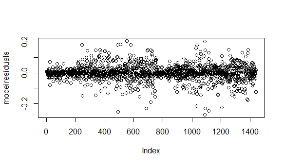
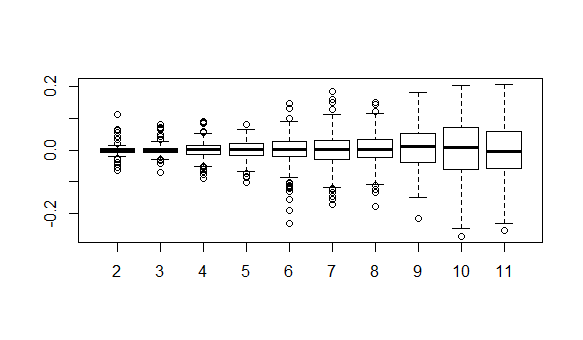
Edit 1: Requested Example residual plots- are any of these a concern. Levene's test, comes back significant.

Residuals are plotted using this code. Time (Obs) is the ordinal factor levels from the data

modelresiduals = residuals(Gama_model)
plot(modelresiduals)
plot(y = modelresiduals, x = Model_data2$Obs)

1. All resids-

2. By time

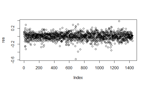
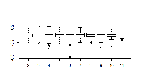
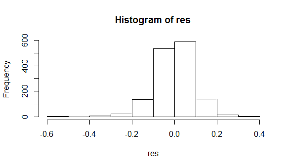
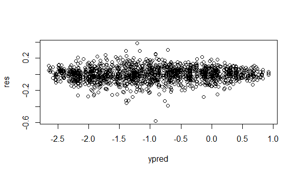
Edit 2 Based on comment suggestions- Patterns look good

ypred = predict(gama_model)
res = residuals(gama_model, type = 'pearson')
plot(ypred,res)
hist(res)
plot(res)
plot(y = res, x = Model_data$Obs)

3. Pearson histograms- based on answer code

4. Pearson vs pred (link scale)- based on answer code

5. All Pearson residual- based on answer code

6. Pearson residual by Time- based on answer code

Answer 1

Are the residuals suppose to be normally distributed...

No. The distribution of $y\vert x$ is assumed to be gamma, and I don't think that $X - \mathbb{E}(X)$ is gamma for $X\sim \text{Gamma}(k,\theta)$. The deviance residuals, on the other hand, should be normal.

is heteroscedasticity a concern like the Gaussian (normal) distribution?

Heteroscedasticity should be observed since the variance changes with the mean.

Here is an example of Gamma regression in R.

library(tidyverse)

#Simulate
set.seed(0)
N <- 250
x <- runif(N, -1, 1)
a <- 0.5
b <- 1.2
y_true <- exp(a + b * x)
shape <- 2
y <- rgamma(N, scale = y_true/shape, shape = shape)

#Model
plot(x,y)
model <- glm(y ~ x, family = Gamma(link = "log"))
summary(model)

#Deviance residuals
ypred = predict(model)
res = residuals(model, type = 'deviance')
plot(ypred,res)
hist(res)

#Deviance GOF

deviance = model$deviance
p.value = pchisq(deviance, df = model$df.residual, lower.tail = F)
# Fail to reject; looks like a good fit.

For more on GLMs, I would recommend Extending the Linear Model by Faraway.

Answer 2

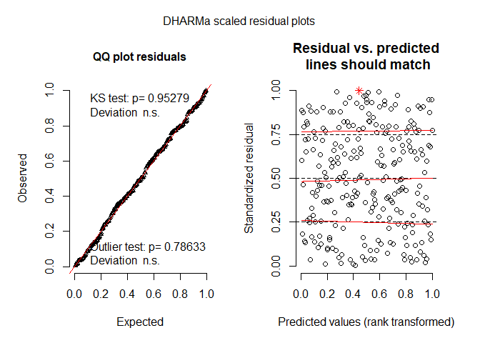
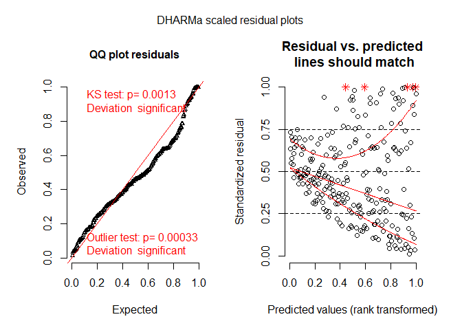
A nice approach for checking the fit of your assumed model to the data, accounting for features, such as, over-dispersion, non-normality, zero-inflation is the simulated scaled residuals provided by the DHARMa package. If your assumed model is correct, these residuals should have a uniform distribution. You can find more details on the procedure they are defined and used in the vignette of the package.

As an example, using the simulated example above, I compare below the fit of the Gamma model to the fit of the wrong normal model:

set.seed(0)
N <- 250
x <- runif(N, -1, 1)
a <- 0.5
b <- 1.2
y_true <- exp(a + b * x)
shape <- 2
y <- rgamma(N, scale = y_true / shape, shape = shape)

gamma_model <- glm(y ~ x, family = Gamma(link = "log"))
normal_model <- glm(y ~ x, family = gaussian())

library("DHARMa")
check_gamma_model <- simulateResiduals(fittedModel = gamma_model, n = 500)
plot(check_gamma_model)

check_normal_model <- simulateResiduals(fittedModel = normal_model, n = 500)
plot(check_normal_model)

Answer 3

For checking the deviance goodness-of-fit statistic for a Generalized Linear Model like a Gamma Regression Model I recommend to follow the instructions on slide 18/19 of Technical University Munich respectively on slide 104 of Technical University Graz.

That is, if dispersion parameter disp can not be assumed to be '1', the residual deviance test, i.e. calculating the p-value, should be applied on the scaled deviance, since the scaled statistic follows the chi square distribution (as outlined in the cited slides), e.g.:

p.value = pchisq(myModel$deviance/summary(myModel$disp), df = myModel$df.residual, lower.tail = F)