Why is Kullback-Leilbler divergence a better metric for measuring distance between two probability distributions than squared error? [duplicate]

Question

I know that KL-divergence is a metric that is more suitable when we want to measure the distance between numbers which a probability form. However, I am still confused what is the benefit of using KL-divergence rather than squared error between probability numbers.

I appreciate if someone can explain this in simple words.

Answer 1

Overview:

• KL-Divergence is derived from the Shannon entropy.
• The Shannon entropy is the amount of information contained in a signal X with distribution $\mathrm{P}(X)$.
• The cross entropy is the information contained in a signal X when we encode it with an estimated distribution $\mathrm{Q}(X)$ instead of its true distribution $\mathrm{P}(X)$.
• The KL-Divergence is the difference in information between the "true" Shannon entropy and the "encoded" cross-entropy.
• The KL-Divergence is asymmetric, because if we gain information by encoding $\mathrm{P}(X)$ using $\mathrm{Q}(X)$, then in the opposite case, we would lose information if we encode $\mathrm{Q}(X)$ using $\mathrm{P}(X)$. If you encode a high resolution BMP image into a lower resolution JPEG, you lose information. If you transform a low resolution JPEG into a high resolution BMP, you gain information. The same applies when you encode a probability distribution $\mathrm{P}(X)$ using $\mathrm{Q}(X)$, or do the opposite. So the property: $$D_\text{KL}(\mathrm{P} \parallel \mathrm{Q}) \neq D_\text{KL}(\mathrm{Q} \parallel \mathrm{P})$$ is in fact desirable, because it expresses the fact that the information is lost one way and gained the other when we use KL-Divergence as a measure of similarity.
• The squared error on the other hand, is symmetric: $$SSE(P,Q) = SSE(Q,P)$$ so the intuitive notion that information will be lost in one direction and gained in the other isn't properly expressed if we use the $SSE$ as a measure of similarity.

---

Details:

To understand KL-divergence, first you need to understand the concept of Shannon entropy:

$$I(X) = -\sum_{i=1}^n {\mathrm{P}(x_i) \log \mathrm{P}(x_i)}$$

The Shannon entropy $I(X)$ is a measure of how much information is contained in a signal $X \in \{x_1,x_2,...,x_n\}$ that is characterized by the distribution $\mathrm P(x_i)$.

In other words, knowing that the probability distribution of $X$ is $\mathrm P(x_i)$ how much information do I learn or gain, when after performing an experiment, I find that the results is $X = x_i$.

To see this consider the case where $\mathrm P(x_i)=1$ for some $x_i$, and 0 for all others. So the event $X = x_i$ was always expected (it is a certain event), and we learn nothing from performing the experiment, hence in this case $X$ has zero information. If you do the math, you will see that in this case, $I(X) = 0$.

If on the other hand, if $\mathrm P(x_i)=\frac{1}{n}$ for all i, i.e we have a uniform distribution and any value of $X = x_i$ is equally likely, the we have the maximum possible value for $I(X)$, given the set $X$.

Now let's define the cross-entropy, which is how much information is in $X$, if I model $X$ with a simulated distribution $\mathrm{Q}(x_i)$ instead of the true distribution $\mathrm{P}(x_i)$:

$$ H(P,Q) = -\sum_{i=1}^n {\mathrm{P}(x_i) \log \mathrm{Q}(x_i)}$$

To simplify, we will write $I(P)$ instead of $I(X)$, since the set $X$ doesn't change. Now you can look at the KL-divergence, which is the difference in information between the case where we use the true distribution $\mathrm{P}(x_i)$ to represent our signal, and a simulated distribution $\mathrm{Q}(x_i)$:

$$D_\text{KL}(\mathrm{P} \parallel \mathrm{Q}) = H(P,Q) - I(P)$$

Now let's fill in the terms:

$$D_\text{KL}(\mathrm{P} \parallel \mathrm{Q})= -\sum_{i=1}^n {\mathrm{P}(x_i) \log \mathrm{Q}(x_i)} + \sum_{i=1}^n {\mathrm{P}(x_i) \log \mathrm{P}(x_i)}$$

And then simplify:

$$D_\text{KL}(\mathrm{P} \parallel \mathrm{Q})= -\sum_{i=1}^n {\mathrm{P}(x_i) (\log \mathrm{Q}(x_i)} - \log \mathrm{P}(x_i))$$

Which in turn leads to:

$$D_\text{KL}(\mathrm{P} \parallel \mathrm{Q}) = -\sum_{i=1}^n \mathrm{P}(x_i) \log\left(\frac{\mathrm{Q}(x_i)}{\mathrm{P}(x_i)}\right)$$

How is this different from using the squared error? Consider the squared error that we have when we estimate $\mathrm{P}(x_i)$ using $\mathrm{Q}(x_i)$:

$$ SSE(P,Q) = \sum_{i=1}^n (\mathrm{P}(x_i) - \mathrm{Q}(x_i))^2 $$

This quantity is symmetrical:

$$SSE(P,Q) = SSE(Q,P)$$

The KL-Divergence is not symmetrical:

$$D_\text{KL}(\mathrm{P} \parallel \mathrm{Q}) \neq D_\text{KL}(\mathrm{Q} \parallel \mathrm{P})$$

---

Numerical example in R:

library(LaplacesDemon) #Use this library for the KLD function
n=10
p=1/2
x=0:10
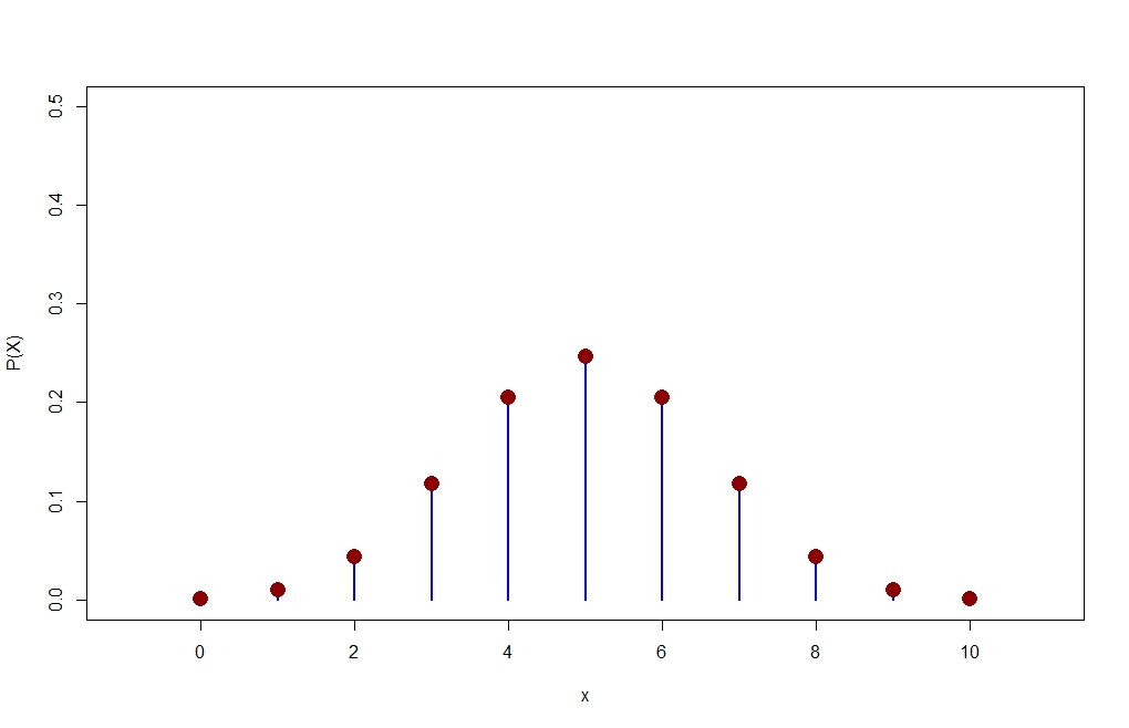
P=dbinom(x,size=n,prob=p)
plot(x,P,type="h",xlim=c(-1,11),ylim=c(0,0.5),lwd=2,col="blue",ylab="P(X)")
points(x,P,pch=16,cex=2,col="dark red")

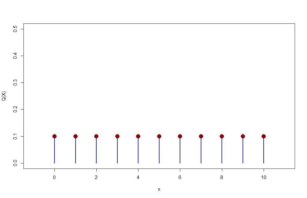
    Q = dunif(x, min=0, max=10, log = FALSE)
    plot(x,Q,type="h",xlim=c(-1,11),ylim=c(0,0.5),lwd=2,col="blue",ylab="Q(X)")
    points(x,Q,pch=16,cex=2,col="dark red")

  > P
 [1] 0.0009765625 0.0097656250 0.0439453125 0.1171875000 0.2050781250
 [6] 0.2460937500 0.2050781250 0.1171875000 0.0439453125 0.0097656250
 [11] 0.0009765625
 > Q
 [1] 0.1 0.1 0.1 0.1 0.1 0.1 0.1 0.1 0.1 0.1 0.1   
 > KLD(P,Q)
 ...
 $sum.KLD.px.py  #This is KL-D(P||Q) 
 [1] 0.5219417
 $sum.KLD.py.px
 [1] 1.077474    #This is KL-D(Q||P)