Isolation Forest Worked Example
First, I remark that there are differences between how different packages implement the isolation forest, and there are also extensions (e.g. extended isolation forest) to the original algorithm.
To write this post I referenced the original paper and the Python scikit learn implementation. In the Python scikit learn implementation they shift and negate the anomaly score, compared to the original paper, therefore don’t be surprised if the scores you get from that package do not match what you get by hand - see this helpful post.
I don’t want to get bogged down in different implementation details, and my aim for this post is just to cover the general procedure.
Motivation - Anomalies are easier to isolate
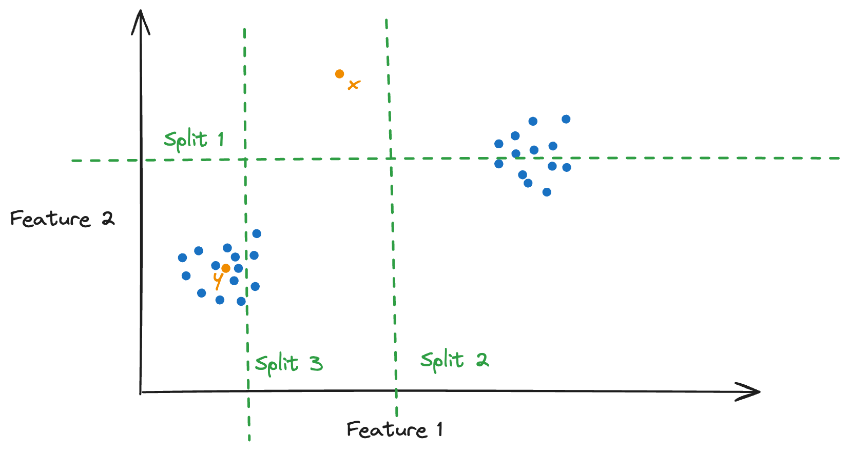
The idea is that if we randomly selected features from our dataset, and then split those features at a random point, then on average the more anomalous points would be ‘easier’ to isolate from the rest of the points. (Easier meaning fewer splits).
See the drawing below for an example:

Loosely speaking, we can see that the point $x$ is “easier” to isolate than the point $y$.
The dashed lines show examples of what some splits might look like this. In this example the point $x$ has already been isolated after the second split.
Roughly Speaking How Does The Algorithm Work?
The first part of the algorithm is to create isolation trees.
A feature is randomly selected, and then a value for that feature is selected uniformly at random between the min and max values. This then creates a split, and the data points are partitioned to the left or right of this split. This process repeats on each side of the split. Hopefully you can imagine how this process can be represented by a tree, but if not see the detailed example below. The tree may terminate when all points are isolated or when the tree depth reaches some threshold.
We can construct multiple isolation trees and then ensemble them together in an isolation forest. (Note that typically the trees are built on a subsample of the data. For simplicity in the small worked example below I use the full dataset to build the trees)
Each data point is assigned an anomaly score, based on how “easy” it is to isolate. Loosely speaking think of the average depth over all trees in the forest for this point to be isolated, and then normalised in such a way as to get a score (say between 0 and 1, although this can vary based on implementation). See the worked example below for more details.
Worked Example - The Trees
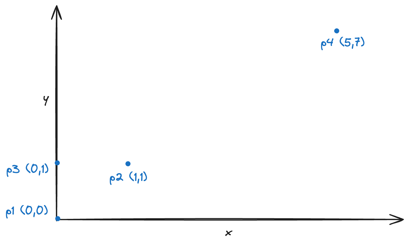
Suppose we have two features $x$ and $y$, and the data points $p_1=(0,0)$, $p_2=(1,1)$, $p_3=(0,1)$ and $p_4=(5,7)$.
See diagram below.

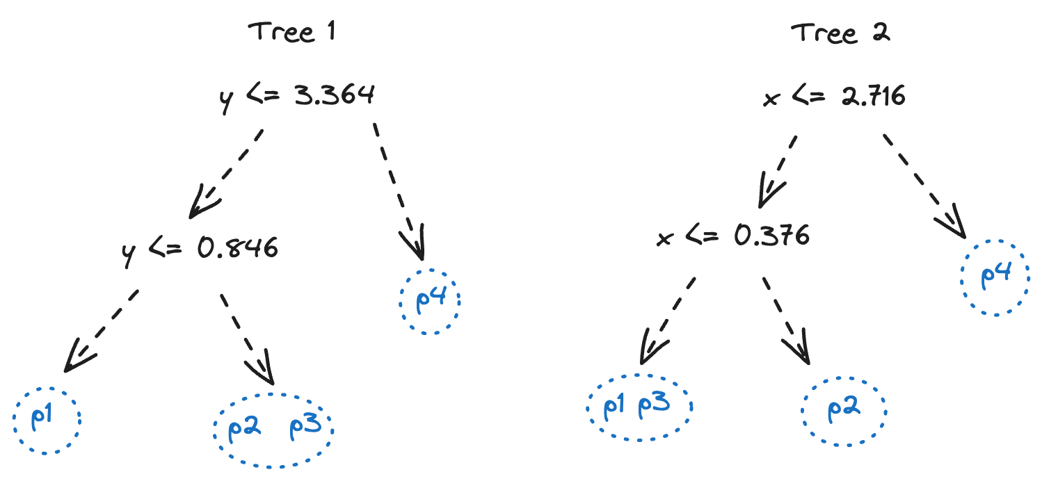
We will create an isolation forest with two trees. I created the trees with scikit learn.
See the diagram below.

At each stage in the tree you can see how the points are split. For example in tree 1, with the condition $y \leq 3.364$, the points $p_1$,$p_2$,$p_3$ move to the left and $p_4$ moves to the right, this isolates $p_4$ as it is the single point in this leaf.
The tree terminates before all points are isolated, for example in tree 1 the points $p_2$ and $p_3$ are not isolated.
Notes:
- The maximum depth of a tree is set by $\text{ceiling} (log_2(n))$, where $n$ is the number of data points used to build the tree, in this case $n=4$ so the trees have depth at most $2$. (With so few data points we will not do any sub sampling.)
- It just happened that one tree only used the feature $x$ and the other only used the feature $y$, this is a coincidence and not a requirement.
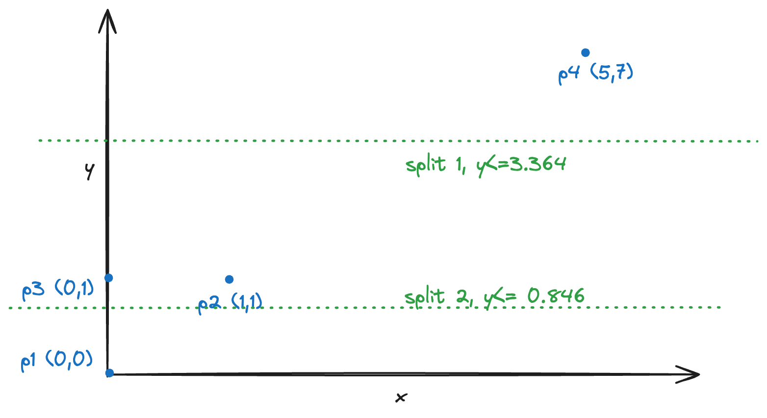
The diagram below shows the splits corresponding to tree 1.

Worked Example - Scoring
The formula used to get the anomaly score is $$ s(p,n) = 2^{\frac{-E(h(p))}{c(n)}}.$$ This will give a score between $0$ and $1$.
Points with scores close to $1$ are consider anomalous while points with scores closer to $0$ are considered normal (typical).
In this formula $p$ is the data point you are scoring and $n$ is the total number of data points. $E(h(p))$ is the average path length of the data point $p$ across all trees in the forest - this is the number of edges the point traverses in a tree on average before it gets isolated.
$c(n)$ is the normalising factor, which is the average path length of an unsuccessful search in a Binary Search Tree (BST).
It depends on the number of data points $n$ and is calculated using the formula:
$$c(n) = 2H(n-1) - \frac{2(n-1)}{n}.$$
Here, $H(i)$ is the harmonic number which can be approximated as
$$ln(i)+0.5772156649 \text{(Euler's constant)}$$
For instance $c(4) \approx 1.852$
Note that in the scikit learn implementation we have, $c(1)=0$, $c(2)=1$. I will follow this in the example below.
For each point, we will calculate the path length in each tree, and the average over all trees in the forest.
$p_4$ is the easiest, in both trees it has a path length of $1$ and is isolated, and so the average is $1$.
The other points are slightly harder, this is because they are not isolated by the time the tree terminates.
In the case that you have multiple points in a leaf node - say $m$ points remaining together in the node, then we add a correction factor to the path length. The correction factor is $c(m)$ (perhaps think of this as accounting for the average difficulty of isolating these points further).
So for $p_1$, in tree 1 it is isolated with a path length of 2. In tree 2, after a path length of 2 it is still not isolated, there are 2 points left in the node, so the path length is $2 + c(2)$. See above that $c(2)=1$, so we write down a path length of 3 for the point $p_1$ in tree 2.
Point $p_2$ is a symmetrical calculation to $p_1$.
Point $p_3$ is not isolated in either tree, in both cases there are two points in the leaf of the tree with it by the time the tree terminates. In both cases the path length is $2 + c(2) = 3$.
We end up with the table below.
| Point $p$ | Tree 1 | Tree 2| $E(h(p))$ average path length over forest|
|---|---|---|---|
|$p_1$|2+1|2|2.5|
|$p_2$| 2+1| 2| 2.5|
|$p_3$| 2+1| 2+1| 3|
|$p_4$| 1| 1| 1|
We calculated $c(4)$ above, and so have all the pieces we need to get the anomaly scores for each data point.
$$s(p_1,4) = 2^{\frac{-2.5}{1.852}} = 0.392$$
$$s(p_2,4) = 2^{\frac{-2.5}{1.852}} = 0.392 $$
$$s(p_3,4) = 2^{\frac{-3}{1.852}} = 0.325$$
$$s(p_4,4) = 2^{\frac{-1}{1.852}} = 0.688$$
In case the links to the diagrams break in future or you are using a screen reader, the splits in tree 1 are first y<=3.364 and then y<=0.846. In tree 2 x<=2.716 and then x<=0.376.

