Why is the intercept in multiple regression changing when including/excluding regressors?

Question

I have a seemingly naive question regarding the interpretation of the intercept in multiple regression. What I found several times is something like this:

The constant/intercept is defined as the mean of the dependent variable when you set all of the independent variables in your model to zero.

https://www.theanalysisfactor.com/interpreting-the-intercept-in-a-regression-model/

https://statisticsbyjim.com/regression/interpret-constant-y-intercept-regression/

But the intercept is changing when including/excluding regressors. As can easily be seen here:

summary(lm(mpg ~ 1, data=mtcars))
Coefficients:
            Estimate Std. Error t value Pr(>|t|)    
(Intercept)   20.091      1.065   18.86   <2e-16 ***


summary(lm(mpg ~ disp, data=mtcars))
Coefficients:
             Estimate Std. Error t value Pr(>|t|)    
(Intercept) 29.599855   1.229720  24.070  < 2e-16 ***
disp        -0.041215   0.004712  -8.747 9.38e-10 ***

summary(lm(mpg ~ disp + hp, data=mtcars))
Coefficients:
             Estimate Std. Error t value Pr(>|t|)    
(Intercept) 30.735904   1.331566  23.083  < 2e-16 ***
disp        -0.030346   0.007405  -4.098 0.000306 ***
hp          -0.024840   0.013385  -1.856 0.073679 .  

So when in my last model, disp and hp are zero, the mean should be 30.7?! Obviously there's a distinction between "being zero" and "being included in the model/estimation".

My professor told me, the interpretation of the intercept in multiple regression is not the expected mean, but the conditional mean.

What does this mean? What is going on here? Thank you

Answer 1

In addition to @DaveT's helpful answer, here are a few more clarifications regarding the estimated intercepts in your models.

Model 1

The (true) intercept in your first model

lm(mpg ~ 1, data=mtcars)

represents the mean value of mpg for all cars represented by the ones included in this data set, regardless of their displacement (disp) or horse power (hp). In this sense, the (true) intercept is simply the unconditional mean of mpg. Based on the data, its value is estimated to be 20.091.

Model 2

The (true) intercept in your second model:

 lm(mpg ~ disp, data=mtcars)

represents the mean value of mpg for all cars represented by the ones included in this data set which share the same displacement (disp) value of 0. This intercept is estimated from the data to be 29.599855. Because displacement is a measure of the engine size of a car, it doesn't make sense that you would have a car with a displacement of 0, suggesting that the intercept interpretation in this model is meaningless in the real world.

To get a meaningful interpretation for the intercept in your second model, you could center the disp variable around its observed mean value in the data (presuming disp has an an approximately normal distribution) and re-fit the model:

disp.cen <- mtcars$disp - mean(mtcars$disp)


lm(mpg ~ disp.cen, data=mtcars)

In the re-fitted second model, the intercept will represent the mean value of mpg for all cars represented by the ones included in this data set which have a "typical" displacement (disp). Here, a "typical" displacement means the average displacement observed in the data.

Model 3

The (true) intercept in your third model:

 lm(mpg ~ disp + hp, data=mtcars))

represents the mean value of mpg for all cars represented by the ones included in this data set which share the same displacement (disp) value of 0 and the same horse power (hp) value of 0. This intercept is estimated from the data to be 30.735904. Because displacement is a measure of the engine size of a car and horse power is a measure of the engine power of a car, it doesn't make sense that you would have a car with a displacement of 0 and a horse power of 0, suggesting that the intercept interpretation in this model is meaningless.

To get a meaningful interpretation for the intercept in your third model, you could center the disp variable around its observed mean value in the data (presuming disp has an an approximately normal distribution), center the hp variable around its observed mean value in the data (presuming hp has an an approximately normal distribution), and then re-fit the model:

disp.cen <- mtcars$disp - mean(mtcars$disp)

hp.cen <- mtcars$hp - mean(mtcars$hp)

lm(mpg ~ disp.cen + hp.cen, data=mtcars))

In the re-fitted third model, the intercept will represent the mean value of mpg for all cars represented by the ones included in this data set which have a "typical" displacement (disp) and a "typical" horse power (hp). Here, a "typical" displacement means the average displacement observed in the data, whereas a typical horse power means the average horse power observed in the data.

Addendum

The word expected is synonimous with the word mean in this answer. Thus, the expected value of the variable mpg is the same as the mean (or average) value.

There are two types of mean values for the mpg variable - unconditional and conditional.

The unconditional mean of mpg refers to the mean value of mpg across all cars represented by the ones in the dataset, regardless of their other caracteristics (e.g., disp, hp). In other words, you would mix together all cars represented by the ones in your data - those with high disp and high hp, those with high disp and low hp, etc. - and compute their mean mpg value, which is an unconditional mean value (in the sense that it does NOT depend on other car characteristics).

The conditional mean of mpg refers to the mean value of mpg across those cars represented by the ones in the dataset which share one or more caracteristics. You could have:

1. A conditional mean of mpg given disp;

2. A conditional mean of mpg given hp;

3. A conditional mean of mpg given disp and hp.

The conditional mean of mpg given disp refers to the mean value of mpg across all cars represented by the ones in your data set which share the same displacement (disp). Since disp can take multiple values, each of its values gives rise to a different conditional mean of mpg given disp. The model that describes how the conditional mean of mpg given disp varies as a function of the disp values is:

lm(mpg ~ disp, data = mtcars)

This model assumes that the conditional mean of mpg given disp is a linear function of disp.

The conditional mean of mpg given hp refers to the mean value of mpg across all cars represented by the ones in your data set which share the same horse power (hp). Since hp can take multiple values, each of its values gives rise to a different conditional mean of mpg given hp. The model that describes how the conditional mean of mpg given hp varies as a function of the hp values is:

lm(mpg ~ hp, data = mtcars)

This model assumes that the conditional mean of mpg given hp is a linear function of hp.

The conditional mean of mpg given disp and hp refers to the mean value of mpg across all cars represented by the ones in your data set which share the same displacement (disp) and the same horse power (hp). Since disp and hp can both take multiple values, each of their combination of values gives rise to a different conditional mean of mpg given disp and hp. The model that describes how the conditional mean of mpg given disp and hp varies as a function of the disp and hp values is:

lm(mpg ~ disp + hp, data = mtcars)

Of course, you could also have a model like:

lm(mpg ~ disp*hp, data = mtcars)

The first of the above models assumes that disp and hp have independent effects on mpg, while the second assumes that the effect of disp on mpg depends on the effect of hp and the other way around.

Answer 2

Your professor comments concerning the conditional mean is when x meets a particular condition. In this case the intercept is the conditional mean of y when x=0. If x never takes the value of 0, then there is no conditional mean for x=0.

As a simple example let us look at y=(-x+10) for x from 0 to 10. If we fit model to the data with no independent variables then the best prediction for y is the mean of y, in this example y=5 (the intercept).
Let us repeat the model with a single independent variable. The model now is y= 10-x, so thus the intercept is now 10.
So the intercept has change from 5 (with no independent variable) to 10 (with a single variable). If we started with a more complex dataset and as we add terms to the model, the intercept and coefficients will change.

Hopefully this example helps explains why the intercept changes with changes in the model.

Answer 3

Question part 1

The constant/intercept is defined as the mean of the dependent variable when you set all of the independent variables in your model to zero.

In short: The intercept term relates to the prediction based on the fitted model, when all independent variables are set to zero. This prediction may be more or less good based on bias and noise.

What is changing when you include more regressors is that the model has more or less bias, and this will influence the prediction of the intercept.

Example case

Say we model points according to

$$y = 0.5 x^2 +5x+30 + \epsilon$$

with Gaussian noise $\epsilon \sim N(\mu = 0, \sigma^2 = 9)$ and let the parameters $x$ be normal distributed $x \sim N(\mu = -3, \sigma^2 = 2)$

set.seed(1)
x <- rnorm(n=400, mu= -3, sigma = 1.4)
y <- 30 + 5*x + 0.5*x^2  + rnorm(n = 400, mu=0, sigma= 9)

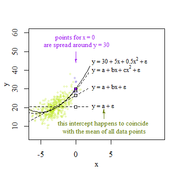
Then it will look like this (I have highlighted the points around $x=0$ in purple):

The model can also be expressed as:

$$y \vert x \sim N(\mu = 0.5 x^2 +5x+30 ,\sigma^2=9) $$

set.seed(1)
x <- rnorm(n=400, mu= -3, sigma = 1.4)
y <- rnorm(n = 400, mu=30 + 5*x + 0.5*x^2, sigma= 9)

which means that the value of $y$ conditional on $x$ is distributed as a normal distribution with mean $\mu = 0.5 x^2 +5x+30$ and variance $\sigma^2=9$.

---

Answer

The constant/intercept is defined as the mean of the dependent variable when you set all of the independent variables in your model to zero.

• This is only for the true quadratic curve $$y = 0.5 x^2 +5x+30$$ which has intercept $30$. Only for the true intercept can we say that the intercept relates to the mean of the data points conditional on the value $x=0$.

  I have marked this point in the figure with a purple square dot.

• For the fitted curves... $$\begin{array}{rcccccccl} y &=& & & &+& {20.1} &+& \epsilon \\ y &=& &+& 2.072 \, x &+&{26.421} &+&\epsilon \\ y &=& 0.3959 \, x^2 &+& 4.4453 \, x &+& \underbrace{{29.2484}}_{\text{intercept terms}} &+& \epsilon \end{array}$$ ...the intercept terms do not refer exactly to the mean of the data (conditional on $x=0$). But more precisely do they refer to the predicted (conditional) mean of the data. And as you can see those predictions can be more or less good due to bias and/or noise.

  I have marked these points in the figure with white square dots.

• In the special case that you fit an intercept only model $y=a+\epsilon$ then the predicted intercept-term $\hat{a}$ will happen to coincide with the unconditional/global mean of the data sample $\hat{a} = \bar{x}$.

  Note that this only means $\bar {x} $ (the mean of some observed sample) is a predictor for the true mean of the entire population (it is not equal to it).

Question part 2

So when in my last model, disp and hp are zero, the mean should be 30.7?! Obviously there's a distinction between "being zero" and "being included in the model/estimation".

The distinction is as following:

• When disp is not in the model
  then the intercept will refer to the mean of mpg for all values of disp.

• When disp is in the model but set at zero
  then the intercept will refer to the mean of mpg for the value of disp=0.

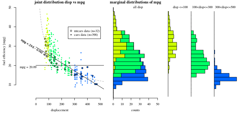
The image below will try to explain intuitively what this 'conditional on disp=0' means.

Note: I have augmented the data with values from another cars set to make the histograms better looking (From: https://github.com/RodolfoViana/exploratory-data-analysis-dataset-cars and http://www.rpubs.com/dksmith01/cars ).

• On the left you see the joint distribution of mpg and disp.
• On the right (in the margin) you see the marginal distribution of mpg only. This marginal distribution can be split up based on conditions on disp. In this image it is for sketched displacement below 100, between 100 and 300, and between 300 and 500 cubic inches.

The intercept (displacement = 0) would just be another condition (other than the three conditions sketched below). For cars it would not make physical/practical sense to have the regressors set at zero (also note the broken gray line that I added, which is the model $\text{mgp}={270}/{\sqrt{\text{disp}}}$; this is probably a more realistic model and that line will never intercept the y-axis at disp=0). The position of the intercept is arbitrary and you can place it anywhere with a shift of variables (think for instance of the temperature scale where 0 degrees Fahrenheit/Kelvin/Celcius all mean something different).