What is the difference between Empirical and analytical PDF and CDF? More Precisely what would be the difference in their plotting?

Question

I am relatively new to statistics with no statistical background whatsoever, I have an assignment in which i have to plot different distributions in these four manners, i have a gist of empirical PDF and Empirical CDF, but have no clue as to what analytical pdf or analytical cdf is. Also I cant seem to find anything on the internet for them. Any help would be much appreciated

Answer 1

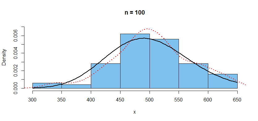
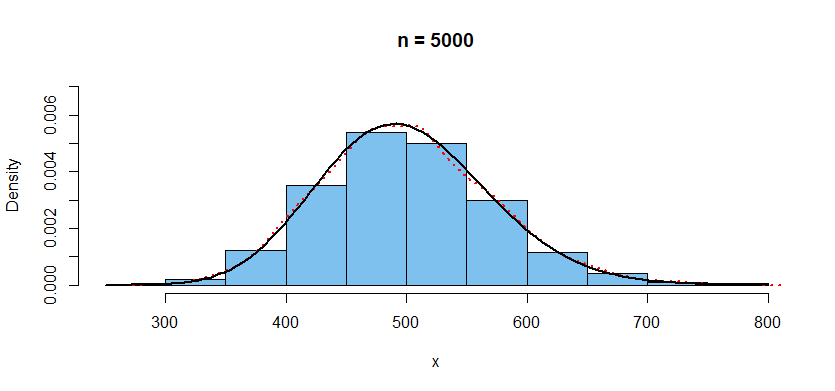
The PDF of a population can be approximated by a histogram (especially if the sample is large) and usually more accurately by a kernel density estimator.

Here are results in R for two samples (of sizes 100 and 5000) from $\mathsf{Gamma}(50, .1).$ The density function of the distribution is shown in black, the KDE as a dotted red curve.

set.seed(1019)
 x = rgamma(100, 50, .1)
 hist(x, prob=TRUE, col="skyblue2", main="n = 100", ylim=c(0,.007))
  lines(density(x), col="red", lwd=2, lty="dotted")
  curve(dgamma(x, 50, .1), add=TRUE, lwd=2)

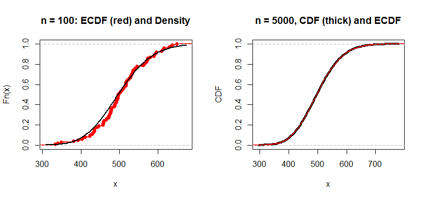
For each of the same two samples, we show plots of the CDF and of the empirical CDF (ECDF). In each panel, the CDF is a thin black curve and the ECDF is shown in red.

To make the ECDF of a sample of size $n:$ (a) sort the observations from smallest to largest, (b) make a jump function with jumps of size $1/n$ at each sorted value. (In case $k$ observations are tied at a common value, the size of the jump there is $k/n.)$

For the larger sample, it is difficult to distinguish the CDF and ECDF at the scale of the graph. For large samples the CDF and ECDF are often much the same. The CDF and ECDF must agree at the far left (where both take the value $0)$ and at the far right (where both take the value $1).$

par(mfrow=c(1, 2))
set.seed(1019);  x = rgamma(100, 50, .1)
plot(ecdf(x), lwd=2, col="red", 
     main="n = 100: ECDF (red) and Density")
curve(pgamma(x, 50, .1), add=TRUE, lwd=2) 
set.seed(1019);  x = rgamma(5000, 50, .1)
  curve(pgamma(x, 50, .1), min(x), max(x), lwd=4, 
     ylab="CDF", main="n = 5000, CDF (thick) and ECDF")
   lines(ecdf(x), col="red", 
         main="n = 5000: ECDF (red) and Density")
par(mfrow=c(1,1))

---

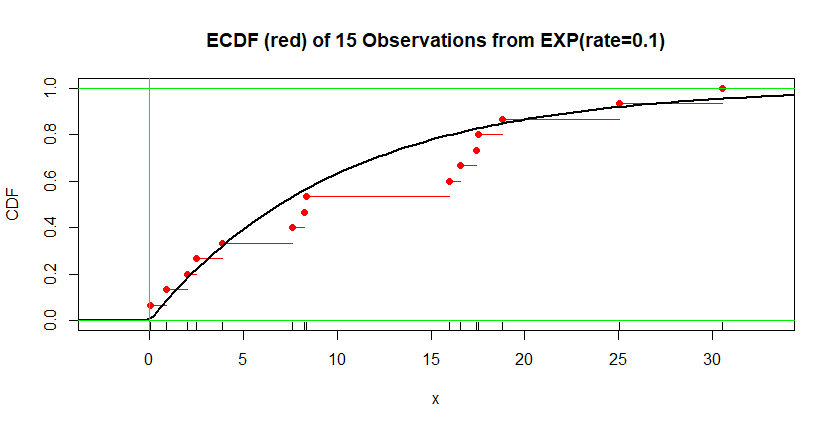
Addendum with a small sample from an exponential population, showing detail of an ECDF plot.

set.seed(1234)
plot(ecdf(w), col="red", ylab="CDF",
    main="ECDF (red) of 15 Observations from EXP(rate=0.1)")
curve(pexp(x, 50, .1), from=-5, to=35, add=T, lwd=2)  
    # mandatory parameter 'x' to specify the curve
rug(w); abline(h=0:1, col="green2"); abline(v = 0, col="green2")