Is there a method to look for significant difference between two linear regression lines

Question

I have two data sets, Fladen A and Fladen B. These are two locations in the North Sea. For each dataset, I have both Age and Height data for a marine mollusk. I have plotted and produced a linear regression line for Age vs height for both datasets.

However, I am not sure what statistical test/R code to use to see if the age height relationship in Fladen A is significantly different to the Age Height relationship in Fladen B.

I have tried anova tests but I do not think this is correct

Answer 1

There are two methods,

1. calculate z statistic between the two means, or
2. fit everything under a linear model and test for the interaction term.

Simulated Dataset

set.seed(123)
df = data.frame(Age=sample(1:100))
df$Height[1:50] = df$Age[1:50] + rpois(50,30)
df$Height[51:100] = 1.3*df$Age[51:100] + rpois(50,30)
df$Fladen = rep(c("A","B"),each=50)

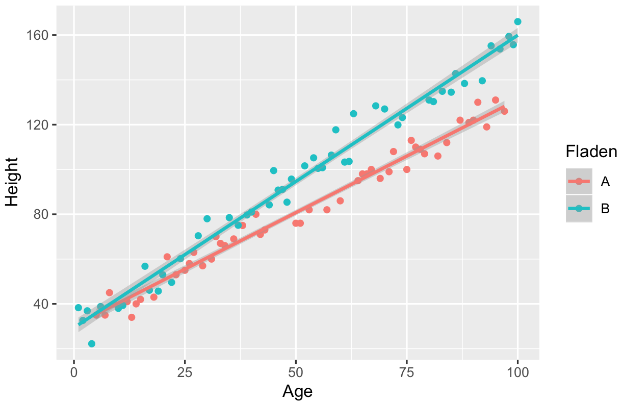
this is how it looks like:

ggplot(df,aes(x=Age,y=Height,col=Fladen)) + geom_point() + geom_smooth(method="lm")

Method 1

You can get a z statistic by finding the difference between the two coefficients, and then dividing by a pooled standard error. See this citation and the formula is like this:

compare.coeff <- function(b1,se1,b2,se2){
return((b1-b2)/sqrt(se1^2+se2^2))
}

where b1, b2 are coefficients of the two lm and se1 and se2 are the standard errors

We fit two linear models:

lm1 = lm(Height ~ Age,data=subset(df,df$Fladen=="A"))
lm2 = lm(Height ~ Age,data=subset(df,df$Fladen=="B"))

b1 <- summary(lm1)$coefficients[2,1]
se1 <- summary(lm1)$coefficients[2,2]
b2 <- summary(lm2)$coefficients[2,1]
se2 <- summary(lm2)$coefficients[2,2]

We calculate the p-value using the z statistic from a normal distribution:

p_value = 2*pnorm(-abs(compare.coeff(b1,se1,b2,se2)))
p_value
[1] 2.747423e-16

Method 2

We combine the information from Fladen A and Fladen B, and run a regression model, the key is to include the Fladen term, to account for overall differences between groups, and Age:Fladen, which accounts for how different the slopes are:

summary(lm(Height ~ Age + Fladen + Age:Fladen,data=df))

Call:
lm(formula = Height ~ Age + Fladen + Age:Fladen, data = df)

Residuals:
     Min       1Q   Median       3Q      Max 
-12.3690  -3.5406  -0.4996   3.4265  13.2879 

Coefficients:
            Estimate Std. Error t value Pr(>|t|)    
(Intercept) 30.28115    1.52481  19.859  < 2e-16 ***
Age          1.00910    0.02641  38.210  < 2e-16 ***
FladenB     -0.93536    2.12168  -0.441     0.66    
Age:FladenB  0.29671    0.03649   8.132 1.49e-12 ***
---
Signif. codes:  0 ‘***’ 0.001 ‘**’ 0.01 ‘*’ 0.05 ‘.’ 0.1 ‘ ’ 1

So the last term, Age:FladenB shows a coefficient of 0.29, meaning the slope (Height vs Age) in Fladen B is .29 more than that in Fladen A, similar to what we simulated.

Note the p-value here is much lower because we use a t-test. So, if your samples size is large, the p-values will be similar, as the t-distribution tends towards normal.

So I would use method 1 or method 2 depending on which one is easier to explain to the interested party..

Answer 2

Do a binary factor for the datasets 0 being for Fladen A and 1 being for Fladen B. From there combine the datasets. You can then run a regression using the binary as an independent variable. If the binary coefficient is significant then the lines are significantly different.

Look at this example pulled from Dr. Garrett Saunders' Statistics Noteboook

lm.2lines <- lm(mpg ~ qsec + am + qsec:am, data=mtcars)

#get the "Estimates" automatically:
b <- coef(lm.2lines)
# Then b will have 4 estimates:
# b[1] is the estimate of beta_0: -9.0099
# b[2] is the estimate of beta_1:  1.4385
# b[3] is the estimate of beta_2: -14.5107
# b[4] is the estimate of beta_3: 1.3214

ggplot(mtcars, aes(y=mpg, x=qsec, color=factor(am))) +
  geom_point(pch=21, bg="gray83") +
  #geom_smooth(method="lm", se=F) + #easy way, but only draws the full interaction model. The manual way using stat_function (see below) is more involved, but more dynamic.
  stat_function(fun = function(x) b[1] + b[2]*x, color="skyblue") + #am==0 line
  stat_function(fun = function(x) (b[1]+b[3]) + (b[2]+b[4])*x,color="orange") + #am==1 line 
  scale_color_manual(name="Transmission (am)", values=c("skyblue","orange")) +
  labs(title="Two-lines Model using mtcars data set")