17
$\begingroup$

I am trying to understand Random Features for Large-Scale Kernel Machines. In particular, I don't follow the following logic: kernel methods can be viewed as optimizing the coefficients in a weighted sum,

$$ f(\mathbf{x}, \boldsymbol{\alpha}) = \sum_{n=1}^{N} \alpha_n k(\mathbf{x}, \mathbf{x}_n) \tag{1} $$

Let $\mathbf{x} \in \mathbb{R}^D$ and let $K < D$. Rahimi and Recht propose a map $\mathbf{z}: \mathbb{R}^D \mapsto \mathbb{R}^K$ such that

\begin{align} \mathbf{w}_j &\sim \mathcal{N}(\mathbf{0}, \mathbf{I}) \\ \hat{k}(\mathbf{x}, \mathbf{y}) &= \sum_{j=1}^{J} \mathbf{z}(\mathbf{x}; \mathbf{w}_j)^{\top} \mathbf{z}(\mathbf{y}; \mathbf{w}_j). \end{align}

Cool so far. Here's what I don't undertstand. Rahimi then claims here that if we plug in $\hat{k}$ into Equation $1$, we get an approximation,

$$ \hat{f}(\mathbf{x}, \boldsymbol{\alpha}) = \sum_{j=1}^J \beta_j \mathbf{z}(\mathbf{x}; \mathbf{w}_j). $$

Question: I don't see how we get to eliminate the sum over $N$. I would have expected:

$$ \hat{f}(\mathbf{x}, \boldsymbol{\alpha}) = \sum_{n=1}^{N} \alpha_n \sum_{j=1}^{J} \mathbf{z}(\mathbf{x}; \mathbf{w}_j)^{\top} \mathbf{z}(\mathbf{x}_n; \mathbf{w}_j). $$

I could possibly rearrange the sums, but I still don't see how we can eliminate the sum over $N$,

$$ \hat{f}(\mathbf{x}, \boldsymbol{\alpha}) = \sum_{j=1}^{J} \mathbf{z}(\mathbf{x}; \mathbf{w}_j)^{\top} \underbrace{\sum_{n=1}^{N} \alpha_n \mathbf{z}(\mathbf{x}_n; \mathbf{w}_j)}_{\beta_j??}. $$

What am I missing?

$\endgroup$

3 Answers 3

9
+25
$\begingroup$

So this kind of looks like a case of notational abuse to me.

Quick Review of Dual Formulation of SVMs and Kernel Trick

For standard, basic vanilla support vector machines, we deal only with binary classification. As is typical, our two class labels will be encoded by the set $\mathcal{Y} = \{+1, -1\}$. I'll also use the notation $[m] = \{1, 2, \dots, m\}$. Our training data set is a sample of size $m$ of the form $S = \{(\mathbf{x}_{i}, y_{i}) \ |\ i \in [m], \ \mathbf{x}_{i} \in \mathbb{R}^{D},\ y_{i} \in \mathcal{Y} \} $.

After reformulating the problem in Lagrange dual form, enforcing the KKT conditions, and simplifying with some algebra, the optimization problem can be written succinctly as: $$\max_{\alpha} \sum_{i = 1}^{m}\alpha_{i} - \frac{1}{2}\sum_{i=1}^{m}\sum_{j=1}^{m} \alpha_{i}\alpha_{j}y_{i}y_{j}(\mathbf{x}_{i}\cdot\mathbf{x}_{j}) \tag{1}\\ \text{subject to}:\qquad\qquad\qquad\qquad\qquad\qquad\qquad\qquad\\ \alpha_{i} \geq 0\ \ \forall i\in [m]\\ \sum_{i=1}^{m}\alpha_{i}y_{i}=0$$

The support vectors are the sample points $\mathbf{x}_{i}\in\mathbb{R}^{D}$ where $\alpha_{i} \neq 0$. All the other points not on the marginal hyperplanes have $\alpha_{i} = 0$.

The Kernel trick comes from replacing the standard Euclidean inner product in the objective function $(1)$ with a inner product in a projection space representable by a kernel function: $$k(\mathbf{x}, \mathbf{y}) = \phi(\mathbf{x}) \cdot \phi(\mathbf{y})\\ \text{where}\ \ \phi(\mathbf{x}) \in \mathbb{R}^{D_{1}}$$ This generalization let's us deal with nonlinearly separable situations since if we take $D_{1} > D$, we can find a linear separator in this higher-dimensional $D_{1}$ space corresponding to a nonlinear separator in our original $D$⁠-dimensional space.

Correcting Notational Abuse

Let's look at these inner products a little more closely. The Euclidean inner product is the familiar sum: $$\mathbf{x}_{i}\cdot\mathbf{x}_{j} = \sum_{t=1}^{D}x_{i,t}x_{j,t} $$

So we see that the objective function $(1)$ really has this $D$ term sum nested inside the double sum. If I write $\phi(\mathbf{x}) = \large{(} \normalsize{\phi_{1}(\mathbf{x}), \phi_{2}(\mathbf{x}), \dots, \phi_{D_{1}}(\mathbf{x})} \large{)} $, then the kernel inner-product similarly looks like: $$\phi(\mathbf{x}_{i})\cdot\phi(\mathbf{x}_{j}) = \sum_{t=1}^{D_{1}}\phi_{t}(\mathbf{x}_{i})\phi_{t}(\mathbf{x}_{j}) \tag{2} $$

So from $(2)$ we are reminded that projecting into this higher-dimensional space means that there are more terms in the inner product. The 'trick' in the kernel trick is that appropriately chosen projections $\phi$ and spaces $\mathbb{R}^{D_{1}}$ let us sidestep this more computationally intensive inner product because we can just use the kernel function $k$ on the points in the original space $\mathbb{R}^{D}$ (for example, as long as the kernel satisfies Mercer's condition).

Ok, everything up to this point has pretty much been reviewing standard material. What Rahimi's random features method does is instead of using a kernel which is equivalent to projecting to a higher $D_{1}$⁠-⁠dimensional space, we project into a lower $K$-dimensional space using the fixed projection functions $\mathbf{z}$ with random weights $\mathbf{w}_{j}$. So rather than having a single projection $\phi(\mathbf{x})$ for each point $\mathbf{x}$, we instead have a randomized collection $\mathbf{z}(\mathbf{x}, \mathbf{w_{j}})$ for $j \in [J]$. In terms of the component notation, earlier we had: $$\phi(\mathbf{x}) = \large{(}\normalsize \phi_{1}(\mathbf{x}), \dots, \phi_{D_{1}}(\mathbf{x} ) \large{)} \tag{3}, $$

whereas now we have: $$ \mathbf{z}(\mathbf{x}, \mathbf{w}_{1}) = \large{(}\normalsize z_{1}(\mathbf{x}, \mathbf{w}_{1}), \dots, z_{K}(\mathbf{x}, \mathbf{w}_{1})\large{)} \\ \vdots \tag{4}\\ \mathbf{z}(\mathbf{x}, \mathbf{w}_{J}) = \large{(}\normalsize z_{1}(\mathbf{x}, \mathbf{w}_{J}), \dots, z_{K}(\mathbf{x}, \mathbf{w}_{J})\large{)}$$

As they allude to in one of the three papers Rahimi places in this trilogy, I forget which one, the components of projection functions of $(4)$ can now be viewed as $J$-dimensional vector valued instead of scalar valued in $(3)$. So now you're replacing your $D_{1}$-dimensional projection with $J$ individual $K$-dimensional projections, and substituted your $D_{1}$ term sum with a $JK$ term sum in each inner product.

So now your inner product is in fact a double sum, over both the $J$ components of each projection and the $K$ dimensions of the space: $$ \hat{k}(\mathbf{x}, \mathbf{y}) = \sum_{t=1}^{K} \sum_{j=1}^{J} \beta_{j}z_{t}(\mathbf{x})z_{t}(\mathbf{y}) \tag{5} $$

Contrast this with the single sum representing the kernel equivalent inner product in $(2)$.

Hopefully tracking each index separately clarified things for you. As for why this is 'efficient,' since the $K$-dimensional projection is lower-dimensional, that's less computational overhead than figuring out the typical higher $D_{1}$ dimensional projection. Also, since you're randomly generating $J$ of these projections, assuming your random generation is computationally cheap, you get an effective ensemble of support vectors pretty easily.

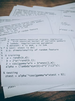
$\endgroup$
6
  • $\begingroup$ This is great, thanks. However, I am confused about $K$. What is $K$ and why isn't it just $J$? Each $z_{\omega_j}$ is really a $D$-vector, since it forms a dot product with a given $\mathbf{x} \in \mathbb{R}^D$. Then $\mathbf{z}_{\boldsymbol{\omega}}(\mathbf{x}) = [z_{\omega_1}^{\top} \mathbf{x}, \dots z_{\omega_J}^{\top} \mathbf{x}]$. $\endgroup$
    – jds
    Commented Dec 20, 2019 at 16:56
  • $\begingroup$ My current understanding is that the efficiency of RFFs is that we can form a matrix $\mathbf{Z}$ that is $N \times J$, and provided $J \ll N$, then linear methods such as computing $\boldsymbol{\beta} = (\mathbf{Z}^{\top} \mathbf{Z})^{-1} \mathbf{Z}^{\top} \mathbf{y}$ is much faster if we did the same computation but with $\mathbf{X}$. For example, matrix inversion in $\mathcal{O}(NJ^2)$ rather than $\mathcal{O}(N^3)$. $\endgroup$
    – jds
    Commented Dec 20, 2019 at 16:59
  • $\begingroup$ I can't edit my first comment, but clearly $\mathbf{z}_{\boldsymbol{\omega}}$ isn't just a vector of dot products but rather the full transformation as described in the paper. $\endgroup$
    – jds
    Commented Dec 20, 2019 at 17:04
  • 1
    $\begingroup$ @gwg I was actually going to expand this answer a little later today, because I realized I was somewhat vague about the efficiency part. In order to really understand the efficiency part, you have to go into the Fourier theory. Given some assumptions on the kernel function you’re trying to approximate, the density of the Fourier basis functions in the function space you’re in implies that a randomly selected collection of basis functions will give you a low error approximation with high probability (a type of PAC learning statement). Will edit my answer to incorporate this aspect. $\endgroup$ Commented Dec 20, 2019 at 17:06
  • $\begingroup$ Rahimi suggests here (youtu.be/4Fz5syoDXXw?t=431) that a representer theorem implies that the decision function $f(x)$ that we want to learn is linear in the high-dimensional space associated with $\varphi(x)$. Therefore, if we have a good approximation of $k(x, y)$, which is equivalent to $\langle \varphi(x), \varphi(y) \rangle)$, then we can assume that our approximation is linear in $z$. $\endgroup$
    – jds
    Commented Dec 22, 2019 at 16:16
4
$\begingroup$

They didn't eliminate data. They replaced the basis functions $k(x,x_n)$ that have data $x_n$ explicitly in them with the ones that don't, i.e. $z(x,w_j)$. Where did the data go? As you noticed, it "went" into the coefficients $\beta_j$.

It's similar to spectral analysis in this regard.

$\endgroup$
3
$\begingroup$

For the linear model $$ f(x, \alpha) = \sum_{n=1}^{N} \alpha_n k(x, x_n) \tag{1} $$

we can write it in matrix form as $$ \hat y = K\alpha \tag{2} $$

where we have some training set of $N$ elements $x_n$ with labels $y_n$, we can collect the $x_n$ in a Gram matrix $K$ such that $K_{ij}=\exp\left(-\gamma\|x_i-x_j\|_2^2\right)$. We have $N$ equations with $N$ unknowns, and we know that the columns of $K$ form a basis, so we can directly solve the linear system $$ \hat \alpha = (K+\lambda I_N)^{-1}y \tag{3} $$ for some regularization hyper-parameter $\lambda \ge 0$. But we still need $N$ evaluations of $k$ to make predictions, and solve an $N \times N$ linear system in some way to get $\alpha$, which is generally expensive.

Rahimi and Recht's early papers show that a random Fourier basis $Z \in [-1,1]^{D \times N}$ is a good approximation: $K \approx Z^\top Z.$ The paper and blog post don't really spell it out, but I think this line in "Reflections on Random Kitchen Sinks" is crucial:

A linear combination of a linear combination is another linear combination, but with this new linear combination has many fewer $(D)$ parameters.

This is somewhat cryptic if you don't already know how random kitchen sinks works. I think the more explicit way to state this is "We can replace solving a large linear system exactly with solving a small linear system approximately, with little loss of precision due to the approximation." We can do this by making the simple and direct substitution $\beta = Z\alpha$ in the original problem, and then solve for $\beta$. Specifically: $$\begin{align} \hat y &= K\alpha \tag{2} \\ &\approx Z^\top Z\alpha \tag{4} \\ &= Z^\top \beta \tag{5} \end{align}$$ for which $\hat \beta$ minimizes square error with regularization $\lambda \ge 0$: $$ \hat \beta = (ZZ^\top + \lambda I_D)^{-1}Zy. \tag{6} $$

In other words, we can just hide the old vector $\alpha$ (with $N$ elements) "under the covers" of the factorization, and work with the more convenient $\beta$ (with $D$ elements). In this way, the problem is reduced to OLS, which is cheaper to solve.

And this is essentially what the authors write in "Random Features for Large-Scale Kernel Machines":

In this set of experiments, we trained regressors and classifiers by solving the least squares problem $$ \min_w \| Z^\top w - y \|_2^2 + \lambda \| w^\top w \|_2^2, $$ where $y$ denotes the vector of desired outputs and $Z$ denotes the matrix of random features. To evaluate the resulting machine on a datapoint $x$, we can simply compute $w^\top z(x)$.

And this result also appears in Rahimi and Recht's guerilla marketing leaflet in "Reflections on Random Kitchen Sinks."

an image depicting the least squares estimator using Fourier basis

This is just OLS with basis expansion! This isn't an SVM (it doesn't maximize a margin or anything), but it is a kernel regression.

You could quite reasonably ask "Why is this interesting? As a matter of principle, it's always true that we can pick some new basis (e.g. polynomials or thin-plate splines, or whatever) for our data, and then estimate a linear model." The key insights in Rahimi and Recht's papers are

  1. The Fourier basis approximates the radial basis function. The explicit feature space of the RBF kernel is infinite, but this approximation can achieve high-quality results with small $D$.
  2. The approximation error is small. Rahimi and Recht show that there are nice probability bounds on the error, and that the approximation gets exponentially better as you increase $D$.

(Of course would never solve this system $(6)$ directly, but instead use a convenient factorization of $Z$, such as $QR$ decomposition or singular value decomposition. Or we could even just use mini-batch methods directly, if the amount of data are truly enormous.)

If we choose the basis dimension $D \ll N$, then we've made some progress to simplifying the task:

  1. We only need $D$ evaluations of our kernel basis, and they're cheap to do.
  2. Decomposing $Z$ is cheaper than solving $K^{-1}y$, especially for large $N$.
  3. We have only $D$ elements in $\beta$, compared to $N$ elements in $\alpha$, so predictions require fewer multiplications.

In the $D \ll N$ setting, the "big idea" is that we don't need to worry about a Gram matrix if we have a good basis. It just so happens that a random Fourier basis is a good basis and also it has a good approximation to RBF.

Of course, you're hardly restricted to $D \ll N$. Rahimi and Recht write

By this third paper, we’d entirely stopped thinking in terms of kernels, and just fitting random basis function to data. We put on solid foundation the idea of linearly combining random kitchen sinks into a predictor. Which meant that it didn’t really bother us if we used more features than data points.

Naturally you can use as rich a basis as you like, even $P \gg N$, and then regularize the result with $\lambda$.


There's also a secret third use-case for random Fourier features. In any case that you need to work with an RBF kernel, but forming the $N\times N$ matrix $K$ is too expensive, it's convenient to work instead with $b^\top K b = b^\top Z^\top Z b$ or $K b = Z^\top Z b$. The approximate factor $Z$ is cheap to compute with a much smaller memory requirement than $K$, and you can choose an expedient order in which to compute the desired product.

$\endgroup$
0

Your Answer

By clicking “Post Your Answer”, you agree to our terms of service and acknowledge you have read our privacy policy.

Not the answer you're looking for? Browse other questions tagged or ask your own question.