The model you discuss in your quesiton can be written as
$$
y = X \beta + F b+e
$$
where $X$ is the matrix with columns equal to $1, x, x^2, x^3,...$ and $F$ is a matrix which columns are obtained by computing the truncated polinomials.
The (penalized) objective function is then:
$$
Q_{p} = \|y - X \beta + F b\|^2 + k\|b\|^{2}
$$
Only the $b$s coefficients are shrunk.
To compute $\beta$ and $b$ we need to solve the following system of penalized normal eqs.:
$$
\left[
\begin{array}{lll}
X'X & X'F \\
F' X & F'F + kI
\end{array}
\right]
\left[
\begin{array}{ll}
\beta\\ b
\end{array}
\right]
=
\left[
\begin{array}{ll}
X'y \\ F'y
\end{array}
\right]
$$
You can compare the system of eqs. above with the one, for example, here https://en.wikipedia.org/wiki/Mixed_model (estimation session). The variance components are $\sigma^2 = var(e)$ and $\tau^2 = var(b)$ and $k = \sigma^{2}/\tau^{2}$.
Why do you have to separate the fixed and random effects this way: You will notice that also in Henderson's mixed model equations the random effects are "penalized" (the $G^{-1}$ term).
What is the random effects distribution in this case: we are assuming that $b \sim N(0, \tau^{2} I)$ and $e \sim N(0, \sigma^{2} I)$
I hope that my answer helps a bit and that I got the notation correct.
Edit
Comment: why do the the tpf part need to be penalized?
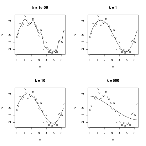
As usual, the penalization controls the trade-off between smoothness and data fitting (see plot below, in which I smooth the same data with fifteen 2nd degree TPF bases and different levels of k-parameter). This is true for all penalized smoothing techniques.

Why do we do all this?
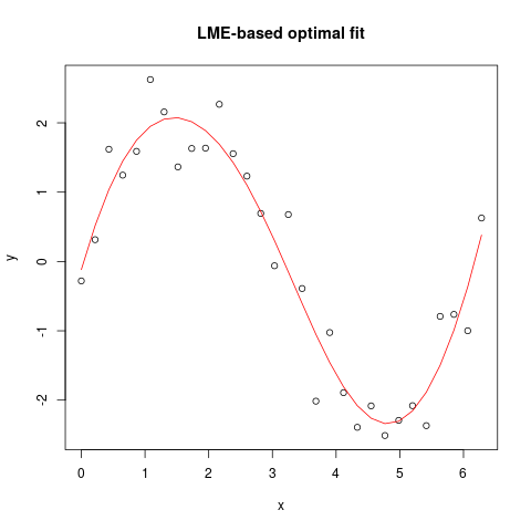
What makes the mixed effect model notation convenient is the fact that the model (including the optimal amount of smoothing) can be computed using standard lmm routines (below I use nlme...notice please that I suppose you have a function to compute the tpf_bases).
# Simulate some data
n  = 30
x  = seq(-0, 2*pi, len = n)
ys = 2 * sin(x)
y  = rnorm(n, ys, 0.5)

# Create bases
Bs = tpf_bases(x, ndx = 10, deg = 2)
X  = Bs$X
Z  = Bs$Z

# Organize for lme
dat     = data.frame(X1 = X[, 2], X2 = X[, 3], y = y)
dat$Z   = Z
dat$all = (1:n) * 0 + 1

# Fit lme
fit = lme(y ~ X1 + X2, random = list(all = pdIdent( ~ Z - 1)), data =
    dat)

# Extract coefficients & get fit
beta.hat  = fit$coef$fixed
b.hat     = unlist(fit$coef$random)
f.hat     = X %*% beta.hat + Z %*% b.hat

# Plot results
plot(x, y, main = "LME-based optimal fit")
lines(x, f.hat, col = 'red')


