Pick a prior for my bayesian generalised linear model with binary outcomes

Question

I need help in my choice of a prior for a bayesian model.

I have data from a set of participants responding to a set of yes/no questions. Answers are correct or incorrect. I suspect some questions are harder than others. I also suspect that some participants are smarter than others. Some of the variance in question difficulty might be explained by question category which I know. Some of the variance in participant smartness might be explained by participant age which I also know.

In a frequentist framework I use a hierarchical logistic generalised linear regression model which predicts response to questions (correct / incorrect) from question category and participant age as population-level predictors with a grouping factor for participants and for questions.

(Age effects might vary across questions and category effects might vary across participants but let's not go there now.)

I'm uncomfortable with the frequentist approach because my participant pool and question pool are both finite. A p value of 0.05 (or whatever) is not trivial to interpret.

As a result I switched to a Bayesian GLMM. This is now easy to do, even for people like me. It has the same description and uses a bernoulli error distribution (recommended by Stan for binary data) and a logit link function. I'm unsure about the choice of a prior for the intercept and for the beta. I don't have great convictions on the prior and want to keep it weakly informative.

1. I first used a noninformative prior, because that's closest to the frequentist mechanics. I can generate the posteriors just fine (based on the WAMBS checklist). But this is generally advised against and, to be honest, I don't actually think that the responses and the effects have infinite variance and can be just about anywhere.
2. I could assume a normal distribution as my prior, or perhaps a student distribution to be a bit stricter. This will be wilfully ignorant of the process that I think is generating my data but it probably won't hurt much.
3. I could use a binomial distribution?
4. I could use a beta distribution? That is apparently the conjugate prior for a Bernoulli likelihood function but I'm not sure how much I should worry about that. Also I'm not sure how to keep such a prior weakly informative but I can look it up.

Answer 1

One trick is to simulate from your priors and see whether you think the models produced this way make a priori sense.

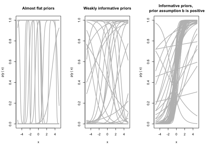
Let's assume we have data $x$ in the range -5 to 5. Below I try three sets of priors for $\alpha, \beta$ in the usual logistic model, increasing in informativeness:

• $\alpha \sim N(0, 100), \beta \sim N(0, 10)$
• $\alpha \sim N(0, 10), \beta \sim N(0, 1)$
• $\alpha \sim N(0, 1), \beta \sim N(1, 1)$

The plot below demonstrates the implied models.

The mostly-flat priors are nonsense. Many of the models predict all 0 or all 1 across the range in question, and where they don't do that they are much too steep in my opoinion. The medium informative priors are perhaps what I would go with in this case, having no strong opinions about direction or steepness of this curve. In the last case I consider what it would look like if I expected $\beta$ to be positive.

This type of thing (ie plotting the model) is difficult to do with many predictors. In this case you could simulate data from the implied models, that is, simulate $\tilde y$ from $$\tilde y_i \sim \mathrm{Bernoulli}( \mathrm{logistic}( \alpha + \beta x_i))$$ and compare with your expectations the $y_i$s, perhaps grouped by some other predictor. If you expect five 0s out of ten then a set of priors whose implied predictions often are all-1 might be too strange.

set.seed(20200228)

par(mfrow=c(1,3))

logistic <- function(z) 1/(1 + exp(-z))

# really wide priors
a <- rnorm(50, 0, 100)
b <- rnorm(50, 0, 10)


plot(NULL, xlim=c(-5, 5), ylim=0:1, xlab = "x", ylab="p(y | x)",
     main = "Almost flat priors")
for (i in 1:50) {
  curve(logistic(a[i] + b[i]*x), add=T, col="grey", lwd=2)
}

# more informative
a <- rnorm(50, 0, 10)
b <- rnorm(50, 0, 1)
plot(NULL, xlim=c(-5, 5), ylim=0:1, xlab = "x", ylab="p(y | x)",
     main = "Weakly informative priors")
for (i in 1:50) {
  curve(logistic(a[i] + b[i]*x), add=T, col="grey", lwd=2)
}


a <- rnorm(50, 0, 1)
b <- rnorm(50, 1, 1)  # note: expecting a positive b now

plot(NULL, xlim=c(-5, 5), ylim=0:1, xlab = "x", ylab="p(y | x)",
     main = "Informative priors, \n prior assumption b is positive")
for (i in 1:50) {
  curve(logistic(a[i] + b[i]*x), add=T, col="grey", lwd=2)
}

^{Created on 2020-02-28 by the reprex package (v0.2.1)}

Answer 2

[edited: Einar's reply goes one step further than what I come up with so I'm picking that one as the answer]

More reading suggests that I was overthinking this. The probability of something happening will be between 0-1, if a factor shifts this probability, the shift will also be between 0-1. If you use a logit link, this is an infinite space, but (-5,5) will cover probabilities between 0.01 and 0.99 and that's probably good enough for most cases in behavioural science.

I'll use a prior distribution that includes these values. The STAN wiki recommends a student t because of concerns about the gaussian.

I'm sure this could be refined in many ways but might work as a first pass. Will check using diagnostics.