I am interested in understanding whether my continuous data (dput code at bottom for reproducibility) are fit better by a linear model (Gaussian distribution) or a gamma distributed model.
I typically use the lme4 package in R (maximum likelihood), but have been toying with the idea of using rstanarm (bayesian) a bit more.
First the ML models:
library(lme4)
library(rstanarm)
library(bayesplot)
library(DHARMa)

lmm <- lmer(Area ~ dB.s + Temp.s + (1 | SITE), data = SPt)
glmm <- glmer(Area ~ dB.s + Temp.s + (1 | SITE),
              family = Gamma(link = "log"), data = SPt)
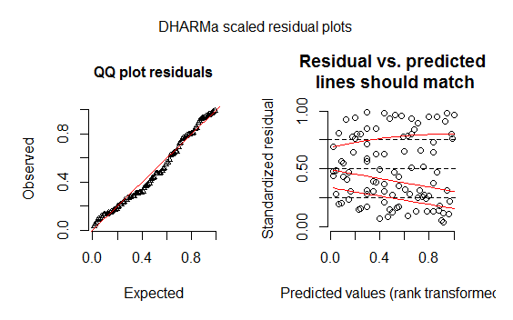
plot(simulateResiduals(lmm))
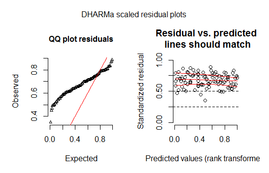
plot(simulateResiduals(glmm))
Just looking at the residual plots, the lmm looks like a much better fit to the data, and the AIC output suggests the same (lower AIC = better):
AIC(lmm,glmm)

    df      AIC
lmm   5 1286.038
glmm  5 1294.297
Now let's try the rstanarm package.
S_lmm <- stan_lmer(Area ~ dB.s + Temp.s + (1 | SITE), data = SPt)
S_glmm <- stan_glmer(Area ~ dB.s + Temp.s + (1 | SITE),
                     family = Gamma(link = "log"), data = SPt)
## All Rhat values of both models are 1.0, indicating good mixing of the chains.
following the loo vignette: https://cran.r-project.org/web/packages/loo/vignettes/loo2-example.html
looL <- loo(S_lmm, save_psis = TRUE)
looL

Computed from 4000 by 97 log-likelihood matrix

         Estimate   SE
elpd_loo   -655.5  6.3
p_loo         6.8  0.9
looic      1311.0 12.5
------
Monte Carlo SE of elpd_loo is 0.1.

All Pareto k estimates are good (k < 0.5).

looGL <- loo(S_glmm, save_psis = TRUE)
looGL

Computed from 4000 by 97 log-likelihood matrix

         Estimate   SE
elpd_loo   -646.6  6.5
p_loo         7.0  0.9
looic      1293.3 12.9
------
Monte Carlo SE of elpd_loo is 0.1.

All Pareto k estimates are good (k < 0.5).
All Pareto k estimates are good, so I think I am okay to go ahead and compare these two:
loo_compare(looL,looGL)
       elpd_diff se_diff
S_glmm  0.0       0.0
S_lmm  -8.9       3.5
Perhaps I am misinterpreting this, but this looks like the stan version of the glmm (Gamma) model (instead of the lmm above) has the best fit to the data (higher number = better in this case). Still following the vignette (link above), comparing LOO-PIT values to generated samples:
yrep <- posterior_predict(S_lmm)
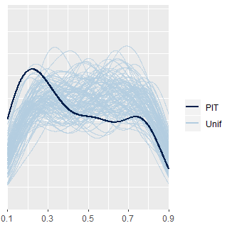
ppc_loo_pit_overlay(SPt$Area, yrep, lw = weights(looL$psis_object))
The model may be a bit underdispersed here, having some excessive zeros, but without a lot of experience with these plots, I am not sure how poor this is.
yrep <- posterior_predict(S_glmm)
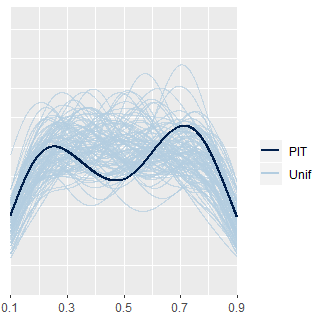
ppc_loo_pit_overlay(SPt$Area, yrep, lw = weights(looGL$psis_object))
The lower end of the glmm looks a bit better (not sure about the hump in the middle).
Am I interpreting these outputs correctly, that the lmm is a better fit with the ML methods (lme4) and the glmm is a better fit with the bayesian methods (rstanarm)? If so, why is this the case?
Data for reproducible example:
SPt<-structure(list(SITE = structure(c(1L, 1L, 1L, 1L, 1L, 1L, 2L,
2L, 2L, 3L, 3L, 4L, 4L, 4L, 4L, 4L, 4L, 4L, 3L, 3L, 3L, 1L, 1L,
1L, 1L, 1L, 1L, 1L, 1L, 1L, 4L, 5L, 5L, 5L, 5L, 5L, 5L, 5L, 5L,
11L, 11L, 11L, 11L, 11L, 11L, 11L, 11L, 11L, 11L, 6L, 6L, 6L,
6L, 7L, 4L, 7L, 7L, 7L, 7L, 12L, 12L, 12L, 12L, 12L, 13L, 13L,
13L, 8L, 8L, 8L, 8L, 8L, 8L, 8L, 10L, 10L, 15L, 14L, 14L, 14L,
14L, 9L, 9L, 9L, 3L, 2L, 2L, 2L, 3L, 3L, 2L, 2L, 2L, 12L, 8L,
8L, 8L), .Label = c("CU0", "CU1", "CU2", "CU3", "CU4", "CW1",
"CW2", "FI10", "FI2", "FI4", "FI5", "FI6", "FI7", "FI8", "FI9"
), class = "factor"), dB.s = c(-0.756084718341438, -0.912553673339041,
-0.756084718341438, -0.912553673339041, -0.549545697744603, 0.00122502384695639,
0.551995745438517, 0.551995745438517, 0.539478229038709, -0.975141255338082,
-0.649685828943069, 0.138917704244847, 0.138917704244847, 0.138917704244847,
0.138917704244847, 0.138917704244847, 0.658394634836886, 0.658394634836886,
-1.16916275953511, -0.57458073054422, -0.57458073054422, -0.680979619942589,
-1.22549158333425, -0.893777398739329, -0.0676213163519883, -0.0676213163519883,
-0.19279648035007, -0.19279648035007, -0.0676213163519883, -0.19279648035007,
-0.130208898351029, -0.167761447550454, 1.17787156542893, 1.17787156542893,
1.17787156542893, 1.04643764323094, 1.04643764323094, 0.545736987238613,
0.545736987238613, 0.332939208441874, 0.332939208441874, 0.345456724841681,
0.345456724841681, 0.345456724841681, 0.345456724841681, 0.345456724841681,
0.345456724841681, 0.345456724841681, 0.345456724841681, -0.0551037999521799,
0.282869142842641, 0.282869142842641, -0.0989151073515087, 0.5269607126389,
0.0512950894461898, 0.35797424124149, 0.35797424124149, 0.501925679839284,
0.501925679839284, 0.126400187845038, 0.126400187845038, 0.126400187845038,
-0.00503373435294734, -0.249125304149207, -0.305454127948344,
-0.305454127948344, -0.180278963950262, -0.267901578748919, -0.480699357545658,
-0.480699357545658, -0.480699357545658, -0.480699357545658, -0.230349029549495,
-0.230349029549495, 0.401785548640819, 0.589548294637941, 0.0262600566465731,
0.470631888839763, 0.401785548640819, 0.126400187845038, 0.126400187845038,
0.00748378204686102, 0.639618360237174, 0.639618360237174, -1.63231086632801,
-0.0363275253524678, -0.0363275253524678, -0.174020205750358,
-0.148985172950741, -1.11283393573597, -0.236607787749399, 0.320421692042066,
-0.205313996749878, -0.286677853348631, 0.239057835443313, 0.239057835443313,
0.239057835443313), Temp.s = c(-0.198220313123015, -0.557916086050254,
-0.198220313123015, -0.557916086050254, 0.0874204477309688, 0.20379260956037,
-0.145323875927833, -0.145323875927833, -0.430964636781816, -0.56849537348929,
-0.251116750318197, -0.642550385562545, -0.642550385562545, -0.642550385562545,
-0.642550385562545, -0.642550385562545, -0.642550385562545, -0.642550385562545,
-0.684867535318691, -0.684867535318691, -0.684867535318691, -0.6002332358064,
-0.557916086050254, -0.557916086050254, -0.621391810684472, -0.621391810684472,
-0.462702499098926, -0.462702499098926, -0.621391810684472, -0.462702499098926,
0.457695508097244, -0.621391810684472, -0.631971098123509, -0.631971098123509,
-0.631971098123509, -0.737763972513873, -0.737763972513873, -0.864715421782311,
-0.864715421782311, 0.6481226819999, 0.6481226819999, 0.6481226819999,
0.6481226819999, 0.6481226819999, 0.6481226819999, 0.6481226819999,
0.6481226819999, 0.6481226819999, 0.6481226819999, 0.552909095048572,
0.806811993585447, 0.806811993585447, 0.859708430780629, 0.859708430780629,
0.32016477138977, 0.679860544317009, 0.679860544317009, 1.02897702980521,
1.02897702980521, 0.425957645780135, -0.219378888001088, 0.425957645780135,
-0.219378888001088, 0.595226244804718, 0.383640496023989, 0.383640496023989,
0.394219783463026, 0.119158310048078, 0.0451032979748232, 0.0451032979748232,
0.0451032979748232, 0.0451032979748232, -0.388647487025671, -0.388647487025671,
0.468274795536281, -0.0924274387326505, -0.304013187513379, 0.0556825854138594,
-0.293433900074343, -0.0289517140984317, -0.0289517140984317,
0.50001265785339, 0.0133654356577138, 0.0133654356577138, -0.293433900074343,
1.00781845492714, 1.00781845492714, 0.690439831756046, -0.251116750318197,
-0.103006726171687, 0.256689046755552, -0.325171762391452, 0.595226244804718,
-0.177061738244942, -0.430964636781816, -0.430964636781816, -0.430964636781816
), Area = c(205.849913383358, 1062.818937407, 337.910550123144,
535.843159145604, 317.637329654352, 773.064126911591, 301.068546437375,
168.859119942524, 254.242114406942, 378.11692072456, 364.829384950198,
298.957412667524, 228.018365593874, 292.623569178805, 447.169350303542,
926.007918050677, 481.372105142623, 131.743944565349, 831.000265719896,
891.805163211596, 501.640404306523, 248.286664757774, 839.867646604103,
860.135945768002, 339.494010995323, 204.709821555389, 648.585573244797,
507.974247795241, 392.381604126125, 784.129823903378, 618.893752757189,
374.963534532148, 175.732839060179, 141.371669411541, 270.176968208722,
61.0647072041516, 235.619449019234, 323.584043319749, 291.382718620453,
241.706284785565, 312.588469032184, 400.356713791849, 828.595062384308,
203.418124319939, 588.852273007237, 235.423099478385, 417.046424764045,
292.168116783851, 499.513231920777, 530.929158456675, 71.4712328691678,
385.630498228147, 223.053078404875, 477.522083345649, 758.498276301086,
554.294753817749, 172.787595947439, 501.869426410969, 670.730031541421,
199.491133502952, 100.074727121756, 286.670329640069, 228.018365593874,
240.331837999619, 386.415896391545, 829.380460547705, 354.214571692249,
360.497756999429, 298.254952550181, 599.062449131404, 461.61777053685,
647.953484802895, 697.989552456803, 304.024487458499, 527.787565803085,
637.743308678728, 435.768432023848, 238.761041672824, 431.968125930617,
686.43799480937, 223.053078404875, 619.679150920587, 312.588469032184,
133.517687777566, 1122.1376259541, 202.436376615692, 584.92528219025,
582.765437240907, 334.426936204349, 461.8141200777, 497.20671386442,
144.411631542787, 387.631221509586, 390.164758905073, 454.769962490004,
333.160167506605, 576.379757473404)), row.names = c(2L, 7L, 8L,
11L, 27L, 31L, 45L, 46L, 50L, 56L, 57L, 63L, 66L, 68L, 70L, 72L,
74L, 77L, 78L, 86L, 88L, 91L, 92L, 96L, 98L, 99L, 100L, 102L,
104L, 105L, 108L, 110L, 112L, 113L, 116L, 117L, 119L, 123L, 127L,
128L, 129L, 131L, 132L, 133L, 134L, 135L, 136L, 138L, 139L, 141L,
143L, 144L, 145L, 146L, 147L, 150L, 151L, 153L, 154L, 157L, 163L,
166L, 168L, 173L, 177L, 178L, 181L, 185L, 187L, 188L, 189L, 190L,
192L, 193L, 198L, 199L, 201L, 208L, 212L, 213L, 214L, 216L, 222L,
223L, 226L, 229L, 230L, 231L, 232L, 235L, 241L, 250L, 260L, 277L,
278L, 279L, 280L), class = "data.frame")


simulateResidualscome from, but it looks as if you are evaluating the Gamma mixed model under a Gaussian QQplot. If that is true, of course the fit is going to look bad. Where is this function found? $\endgroup$library(DHARMa)into the code above, wheresimulateResidualscomes from. As far as I know, it is designed to be compatible with different distribution families, but I cannot really say how it works: cran.r-project.org/web/packages/DHARMa/vignettes/DHARMa.html $\endgroup$