Should I use 'median' instead of 'mean' for nonparametric distributions?

Question

I have a dataset that I determined was nonparametric. If I want to do calculations like '% change', and find the average percentage change, should I really find the median percentage change instead of the average? Because it is not-normally distributed?

Answer 1

As pointed already by @Alexis, as dataset is not "parametric" or "non-parametric". Strictly speaking, if we created a dataset using a known simulation setting we could argue that is "parametric" based on the parameters of the simulation but even then it is a bit of stretch.

In a parametric modelling approach, the number of parameters $k$ is fixed with respect to the sample size $N$. (For our simulated data example, if we simulate data from a Gaussian distribution we just care for the mean $\mu$ and standard deviation $\sigma$; that is irrespective of $N$.) In a non-parametric modelling, the number of parameters $k$ is related to the sample size $N$. For example, in a Gaussian Process regression, the errors are assumed to have a multi-variate Gaussian distribution, as we get more data, we get more parameters.

Focusing on how to report "% of change":

1. Plot the data and show the relevant distribution of changes.
2. Both the mean and the median can be valid summaries and both aim to encapsulate the central tendency of our underlying distribution. The median is "more resistant" to abrupt changes than the mean but that in itself is neither good or bad. There are no comments on the size of the data but realistically the larger the dataset, the smaller the small the expected impact of single data-point.
3. Percentage change especially when the two numbers are close to each other approximate the natural log changes (See this excellent CV for more details: Why is it that natural log changes are percentage changes? What is about logs that makes this so?). Does it make more sense to transform these data anyway? Would it make sense to consider winsorization instead?
4. Indeed, using the median instead of the mean is advocated as a "quick fix" when we think that the data is "non-normally distributed". But that's not always right. An obvious counter-example is Poisson-distributed data where the mean is perfectly interpretable as the rate $\lambda$ but the shape for $\lambda < 10$ is obviously not bell-shaped at all.

Answer 2

I think it is best to avoid declarations about 'percentage change' and to use 'change' in weights. If median weight changed from 180 kg to 170 kg after a 3-month program of exercises, then it's clear that the median weight decreased by 10 kg. (If subjects weighed 280 kg to start, then a 10-kg average loss would be a smaller percentage. Would you expect heavier people to lose the same percentage of their weight over 3 months--or to take longer doing that?)

Using R, suppose I have $n = 100$ differences d in weights during an exercise program designed to promote weight loss. $D = $ Before - After.

d = x1 - x2
summary(d)
   Min. 1st Qu.  Median    Mean 3rd Qu.    Max. 
 -9.434   1.307  11.390  10.709  20.622  29.961 
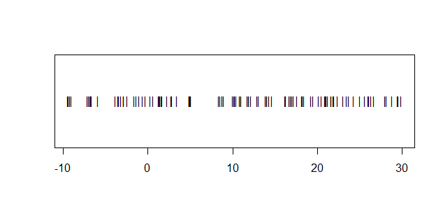
stripchart(d, pch="|")

Not everyone lost weight (one person gained 9.4 kg). The weight losses are not normally distributed according to a Shapiro-Wilk test for normality, which shows a P-value about $0.003 < 0.05.$

shapiro.test(d)

        Shapiro-Wilk normality test

data:  d
W = 0.95792, p-value = 0.002867

A one-sample Wilcoxon test on the differences d shows a negative shift in weights. (P-value near 0.)

 wilcox.test(d)

         Wilcoxon signed rank test 
         with continuity correction

 data:  d
 V = 4530, p-value = 5.497e-12
 alternative hypothesis: true location is not equal to 0

However, the differences show no outliers and no severe skewness, so with $n = 100$ observations, it seems OK to use a paired t test (one-sample t test on differences), as follows. The mean weight loss is significantly different from $0.$

I did 2-sided tests because some weight-loss schemes have turned out to be counterproductive; even if not intended, results might have been in the direction of a weight gain. After an afternoon of punishing exercises, a huge hot-fudge sundae may seem just the thing!

Now, we look at a t test to see that there has been a statistically significant average weight loss of about 10.7 kg. (P-value near 0.)

t.test(d)

        One Sample t-test

data:  d
t = 9.5044, df = 99, p-value = 1.319e-15
alternative hypothesis: true mean is not equal to 0
95 percent confidence interval:
  8.472987 12.944201
sample estimates:
mean of x 
 10.70859 

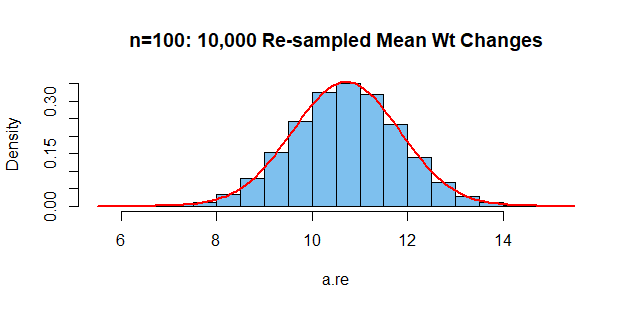
The requirement for using the t test is not that the individual weight changes need to be normal, but that the mean weight change $\bar D$ should be nearly normal. With no outliers, no skewness, and 100 observations, it seems safe to believe that is so.

By re-sampling 100,000 groups of size 100 without replacement from among the d-values, we can get an idea that averages of such values are indeed nearly normal.

set.seed(2020)
a.re = replicate(10^5, mean(sample(d, 100, rep=T)))
hist(a.re, prob=T, col="skyblue2", 
     main="n=100: Re-sampled Mean Wt Changes")
  curve(dnorm(x, mean(a.re), sd(a.re)), add=T, col="red", lwd=2)

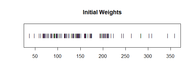
Note: Data for this example were simulated as shown below. In an actual study there could be outliers among the weight changes and overall skewness.

set.seed(607)
x1 = rgamma(100, 5, 1/30)
x2 = x1 - runif(100, -10, 30)

stripchart(x1, pch="|", main="Initial Weights")