Polynom fit with big errors and wrong parameters

Question

I have a question about polynomial fitting with python and I think its a more statistical question.

When I generate code for a polynomial function 3rd order with a not constant offset/error in the $y$-axis and then try to fit a polynom at it with scipy.optimize not only the errors are very big, but also the parameters are completely wrong. I even give the right parameter as starting point to curve_fit. Anyway, if I use a different Method (numpy.polynomial or Fityk) I get the same strange results.

Here is a minimalistic code-example:

import numpy as np
import matplotlib.pyplot as plt
from scipy import optimize, special
import random

x = np.arange(-8,8,1)
y = []
Parameter = [1,2.2,3,-1.54]
for i in range(len(x)):
    off = random.randrange(-50,50,1)/100 #plusminus 0.5
    z = x[i] + off
    tmp = Parameter[0]+Parameter[1]*z+Parameter[2]*z**2+Parameter[3]*z**3
    y.append(tmp)
    

def fit(x,a,b,c,d):
    return a+b*x+c*x**2+d*x**3
params, cov = optimize.curve_fit(fit,x,y,p0=[1,2.2,3,-1.54])
errors = np.sqrt(np.diag(cov))

print(params,errors)    

plt.plot(x,y,'rx',label="datapoints")
plt.plot(x,fit(x,*params),label="optimize-fit")
plt.plot(x,fit(x,*Parameter),linestyle=":",label="original")

plt.legend()
plt.show()

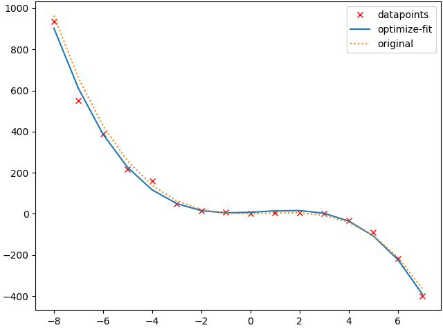
The output is then for example [ 7.52024669 6.46958267 2.08168315 -1.59063913] [9.14611526 3.27003474 0.34030295 0.07992523] and the plot looks like this:

So the fit looks and follows the data points quite good, but the parameters $a$ and $b$ are very off, no matter how many data points there are. Is there a way to make the fit better, or is this a statistical problem I can't quite grasp?

Maybe it's relevant to say that I have real measured data points which behave the same way, but are too odd to take in a minimalistic example. And sorry for the worse than average English.

Answer 1

You're adding noise to your x values, not your y values. Ordinary regression assumes that the only error is in measurement of y, not measurement of x.

for i in range(len(x)):
    off = random.randrange(-50,50,1)/100 #plusminus 0.5
    z = x[i] 
    tmp = Parameter[0]+Parameter[1]*z+Parameter[2]*z**2+Parameter[3]*z**3 + off
    y.append(tmp)

This gives estimated parameters of [ 1.07428852 2.20807026 2.99711762 -1.54046383], which is close to your real parameters. These aren't exact because of the random variation in y.

If you're trying to model random variation in the independent variable x instead of the more usual y, then you're looking for an error-in-variables model.