Matt's trick (reparametrization) makes my models slower, not faster

Question

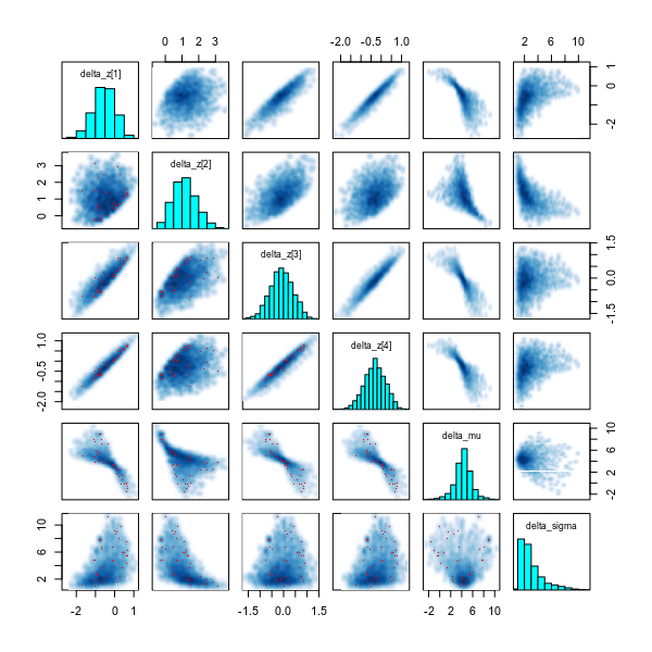
I am currently programming a hierarchical model in Stan. Following the advice from section 22.7 from the Stan manual, I reparametrized my model so it samples the individual differences from a $N(0,1)$ standard normal instead of a $N(\mu,\sigma^2)$ distribution. However, I found the model to be very slow, so I looked at the pairs plot. This plot shows severe funnels in the posterior distribution of the parameters that are sampled with the $N(0,1)$ prior. Also, the posteriors are highly correlated between subjects, which I found very surprising:

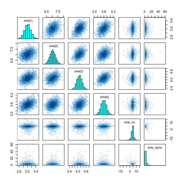
When I looked at the resulting posteriors of the variables, after they are translated from z-scores to the actual values, I found that there are neither funnels, nor the between-subject correlations. So I decided to remove Matt's trick and sample directly from the $N(\mu,\sigma)$ distributions. This sped up my models (from 13 minutes to around 2 minutes), and there are no observable funnels or correlations in the variables:

Here is my model with Matt's trick:

data {
  int<lower=1> N;
  int<lower=1> M;
  vector<lower=0>[N] RT;
  int<lower=1> subj[N];
  vector<lower=0,upper=1>[N] resp_l;     // 1 if the response was on the left, 0 otherwise
  vector<lower=0,upper=1>[N] incomp;     // 1 if the trial was incompatible, 0 otherwiese
  vector<lower=0,upper=1>[N] acc;        // Accuracy: correct (1) or incorrect (0) response
  real<lower=0> NDTMin;
  real<lower=0> minRT;
}

parameters {
  // Group level parameters
  real<lower=0> alpha;                              // Boundary separation
  real<lower=NDTMin,upper=minRT> tau;               // non-decision time
  real<lower=0,upper=1> beta;                       // initial bias
  real delta_mu;                                    // mean drift rate (group level)
  real<lower=0> delta_sigma;                        // variance
  real eta;

  // Individual parameters
  vector[M] delta_z;                               // difference in drift rate for eah subject (z-score)
}

transformed parameters {
  vector[N] beta_trl;   // Beta for each trial
  vector[M] delta;      // Individual drift rate, after conversion from z-score
  vector[N] delta_trl;  // Drift rate in each trial

  // initial offset should mostly depend on handedness etc.
  // i.e. a single offset towards left/right responses
  // therefore, we reverse the beta, if the response was on
  // the left
  beta_trl = beta+resp_l-2*beta*resp_l;

  delta = delta_mu + delta_sigma * delta_z;

  delta_trl = (delta[subj]+incomp*eta) .* (2*acc-1);
}

model {
  alpha       ~ normal(0,1);
  tau         ~ beta(1,1);
  beta        ~ beta(1,1);
  delta_sigma ~ cauchy(0,100);
  delta_mu    ~ normal(0,10);
  eta         ~ normal(0,10);

  // Difference from group mean is in z-score.
  // will be transformed later
  delta_z ~ normal(0,1);

  RT ~ wiener(alpha, tau, beta_trl, delta_trl);
}

In the second model, I just removed the delta as a generated parameter and directly sampled delta as

delta ~ normal(delta_mu,delta_sigma);

Is there something wrong, or is Matt's trick just not working in this case. If it's a problem with Matt's trick that makes it do the opposite of what it is supposed to do (creating funnels instead of removing them), then why is this the case here.

EDIT:

From looking at the distributions again, it seems as $\mu_\delta$ is distributed differently in the two posteriors. But this seems to be mostly in the tails:

             mean se_mean   sd  2.5%   25%   50%   75% 97.5% n_eff Rhat
alpha        1.64    0.00 0.05  1.54  1.60  1.64  1.67  1.74  2388 1.00
beta         0.50    0.00 0.01  0.48  0.49  0.50  0.50  0.51  1947 1.00
delta_mu     4.26    0.05 1.55  0.68  3.47  4.30  5.13  7.47   822 1.01
delta_sigma  3.01    0.07 1.76  1.13  1.78  2.45  3.67  7.93   730 1.00
tau          0.21    0.00 0.00  0.20  0.20  0.21  0.21  0.21  2163 1.00
eta         -0.56    0.00 0.14 -0.82 -0.66 -0.56 -0.47 -0.30  2987 1.00

in the model with Matt's trick, and

             mean se_mean   sd  2.5%   25%   50%   75% 97.5% n_eff Rhat
alpha        1.64    0.00 0.05  1.54  1.61  1.64  1.67  1.74  2136    1
beta         0.50    0.00 0.01  0.48  0.49  0.50  0.50  0.51  4318    1
delta_mu     4.26    0.06 2.06  0.08  3.47  4.37  5.20  8.14  1136    1
delta_sigma  3.59    0.12 3.59  1.11  1.83  2.62  3.99 12.09   927    1
tau          0.21    0.00 0.00  0.20  0.20  0.21  0.21  0.21  2732    1
eta         -0.56    0.00 0.14 -0.82 -0.65 -0.56 -0.47 -0.29  2796    1

in the model without.

Answer 1

It is not unheard of for the centered parameterization to be better. This post on the Stan forums goes into the exact same issue. There it is suggested that

[...] centered actually works better when you have informative data (large N relative to $\sigma$) for a particular group, while non centered is better for uninformative data (small N relative to $\sigma$)

This post, linked from the one above, discusses the issue in terms of estimating a someting in groups of differing size, (ie of differing informativeness) and it is suggested that

[...] you can gather your individual groups into "informative data" and "non-informative data", implement the former with a centered parameterization and the latter with a non-informative parameterization, and see if that improves anything.