Bootstrap vs Wilson score confidence interval

Question

For estimation of the confidence interval of sensitivity and specificity, when I should use the Wilson score and when I should use bootstrapping?

Answer 1

I think that you should use whichever method gives you the best coverage in the region of interest. For the coverage of bootstrapping techniques there is

Mantalos, P. and Zografos, K., 2008. Interval estimation for a  
binomial proportion: a bootstrap approach. Journal of   
Statistical Computation and Simulation, 78(12), pp.1251-1265.

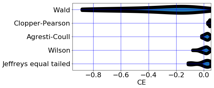
Here's a Python script that identifies the coverage for techniques including the Wilson interval given x, n and CL. It doesn't include any bootstrapping based non parametric techniques but I think it would be better it it did.

Figure 1, coverage error (CE) for different techniques for Interval estimation for a binomial proportion

import statsmodels.api
from rpy2.robjects.packages import importr
binom = importr('binom')
from rpy2 import robjects
import matplotlib.pyplot as plt

n = 10 # samples
x = 10 # positive results
CL = 0.95 # confidence level
print('confidence level: ',CL)

methods = ["'bayes', type='central'",
           "'wilson'",
           "'agresti-coull'",
           "'exact'",
           "'asymptotic'"]
LW = 10 # line width

# CI
low, high = statsmodels.stats.proportion.proportion_confint(x, n, alpha=1-CL, method='jeffreys')
if x == 0: low  = 0
if x == n: high = 1

# CP
step = (high - low) / 31

robjects.globalenv["LV"] = robjects.r(low)
robjects.globalenv["HV"] = robjects.r(high)
robjects.globalenv["SV"] = robjects.r(step)
robjects.globalenv["CV"] = robjects.r(CL)

CP = {}

for method in methods:
    r_string = """library(binom)
    p = seq(LV,HV,SV)
    coverage = binom.coverage(p, 10, conf.level = CV, method=TECHNIQUE)$coverage
    """.replace('TECHNIQUE',method)
    robjects.r(r_string)
    R_C = list(robjects.r['coverage'])
    CP[str(method)] = R_C

R_P = list(robjects.r['p'])

# Coverage Error (CE) = CP - CL
CE = {}
for method in methods:
    CE[str(method)] = [x - CL for x in CP[str(method)]]

# Dict to Lists
labels, data = [*zip(*CE.items())]

# Plots    
font = {'weight' : 'normal',
        'size'   : 22}
plt.rc('font', **font)

# Violin
fig, ax = plt.subplots()
parts = plt.violinplot(data, showextrema=False, vert=False)

for pc in parts['bodies']:
    pc.set_edgecolor('black')
    pc.set_alpha(1)
    pc.set_linewidth(LW)

plt.xlabel('CE')
fig.set_size_inches(8,4)
#plt.xlim([-.05,.05])
plt.xlim([-CL,1-CL])

# Override the method names
labels=(['Jeffreys equal tailed','Wilson','Agresti-Coull','Clopper-Pearson','Wald'])

plt.yticks(range(1, len(labels) + 1), labels)

plt.grid(b=True, which='major', color='b')
plt.show()