Estimation of Sparse Panel Data

Question

There are 1000 students and 100 teachers. Each teacher is given the answer scripts of randomly selected 100 students. So in total 10,000 answer scripts are judged.

Now this is sort of panel data, but lots of missingness. If i want to find which teachers are lenient in grading and which are stricter, what technique can i use.

Imputation shall not work as missingness is around 90%.

The basic way to work this - that comes to me seems to be -

• Define a data structure for assessment:id, teacher id, student id, marks
• Group by students and for each group rank the teachers based on marks
• Compute normalized average ranks for each teachers, normalisation required to accommodate different numbers of assessments done by different teachers
• Then rank the teachers based on this averages or do clustering based on this average ranks to split them in to strict and lenient

How to estimate standard error? What is underlying probability distribution?

Is there a standard methodology to handle such a problem? what if instead of marks, we have categorical variables (grades) like A,B,C,D.

Answer 1

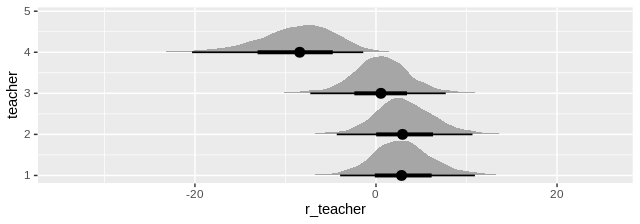
Assuming, there's no problematic bias in how teachers are assigned to students (ideally, you'd have [stratified] random allocation), one standard approach to this would be to fit a random effects model. Let's say that the score is a number on an ordinal scale (i.e. a finite number of discrete values e.g. A, B, C, D, E, F or 1,2,3,4,5,6 or 0,1,2,3,...,15 or whatever various countries use). You could then define an ordinal logistic regression model with a random teacher effect (measures whether teachers tend to give better or lower grades) and a random student effect (measures how good the student is).

E.g. using R and the brms package, an analysis could look like this:

library(tidyverse)
library(brms)
library(tidybayes)

example = tibble(teacher= c(1,1,1,1,1, 2,2,2,2,2, 3,3,3,3,3,3, 4,4,4,4,4,4),
                 student= c(1,2,3,4,6, 2,3,4,5,7, 1,3,4,5,6,7, 1,2,3,5,6,7),
                 grade  = c(1,2,3,5,5, 2,3,4,5,6, 1,3,3,4,5,6, 1,1,1,2,4,4)) %>%
  mutate(grade = ordered(grade, levels=1:6))

# Fit brms ordinal logistic reg. model with default priors (for other options, see below)
brmfit1 = brm(data = example, 
              formula = grade ~ (1 | teacher ) + (1 | student),
              family = cumulative(link = "logit", threshold = "flexible"))

# Look at the random effects (can of course also get full MCMC samples)
ranef(brmfit1)

# Plot model estimates of difficulty of each case
brmfit1 %>%
  spread_draws(r_teacher[teacher, Intercept]) %>%
  ggplot(aes(y = teacher, x = r_teacher)) +
  geom_halfeyeh()

The nice thing about taking this type of Bayesian approach is that getting estimates and credible intervals for the random teacher effects is incredibly straightforward.

This is described e.g. in the brms package documentation, as well as in a publication by its author. See also (shows some options for priors) this post on the Stan discourse page.

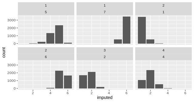
You can in fact also get a reasonable imputation for the teacher-student pairs you do not have data for, e.g. like this:

missing_combinations = expand_grid(teacher=1:4, student=1:7) %>%
  left_join(example, by=c("teacher", "student")) %>%
  filter(is.na(grade)) %>%
  dplyr::select(teacher, student)

# Produces predictions: 
#  rows = a multiple imputation, 
#  columns = a record for which we get a prediction
preds1 = predict(brmfit1,
                 newdata = missing_combinations,
                 summary=FALSE)

preds1 %>%
  as_tibble() %>%
  pivot_longer(cols=starts_with("V"),
               names_to="row", values_to="imputed") %>%
  mutate(rowno = as.numeric(str_extract(row, "[0-9]+$"))) %>%
  left_join(missing_combinations %>% mutate(rowno=1:n()), by="rowno") %>%
  ggplot(aes(x=imputed)) +
  geom_bar() +
  facet_wrap(~teacher + student)

However, note that while different teacher can have different random effects, i.e. one teacher gives consistently higher or lower grades, the “distance” on the logit-scale between grades is the same across teachers. I.e. you are making a proportional odds assumption. If you want to relax assumptions like that one, look into item response theory (IRT), e.g. you could modify an IRT model to say that somehow the IRT model parameters are exchangeable between teachers.

Note: R package versions for some of the key packages that I used in R-3.6.1 for the example were tidyverse_1.2.1, tidybayes_1.1.0, brms_2.10.0, rstan_2.19.2 and Rcpp_1.0.3 (there's now R version 4 and especially tidybayes has been updated a lot since that version).