Root-finding via Robbins-Monro method: A real and simple example

Question

I am looking for a real and simple example for the Robbins-Monro (RM) method, but most of the googled results are theoretical and abstract. To understand the RM, I used a simple function \begin{equation*} f( x) =\frac{1}{1+exp( -0.5x)} -0.5+u=0 \end{equation*} where $\displaystyle x$ is the variable and $\displaystyle u\sim N\left( 0,0.1^{2}\right)$ is noisy variable. The root is 0.

The $\displaystyle x$ is updated via the RM by

\begin{equation*} x_{t+1} =x_{t} -a_{t} f( x_{t}) \end{equation*} where $\displaystyle t$ is the iterative index and $\displaystyle a_{t}$ is the nonnegative 'gain' value which is $\displaystyle a_{t} \varpropto ( 1/t)^{b} ,\ 0.5< b\leqslant 1$.

However, even that simple example, I found it is difficult to get the RM converge to the root. The R code is as follows:

f.error <- function(x){
  1/(1 + exp(-0.5 * x)) - 0.5 + rnorm(n=1,mean=0,sd=0.1)
}
x = 2 # starting value (should not too far away from solution)
dif = Inf
ite = 0
r = x 
b = 0.5
while (dif > 0.0001){
  ite = ite + 1
  a = (1/ite)^b
  x = x - a*f.error(x)
  r = c(r,x) # save results
  if ((ite %% 3) == 0){
    dif = abs(x - r[ite-2])
  }
  print(x)
}
plot(1:length(r),r)

Questions:

1. How to adjust the a and b?
2. How to make the RM perform better?

Answer 1

It seems to be performing just fine.

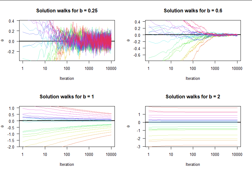
Let's do a small study. The plots below document 10,000 steps of the process of finding the root $\theta$ for four values of $b$ (indicated in their titles) and 20 values of the initial estimate $a$ (randomly chosen at the outset and common to all four panels). The colors indicate the values of $a.$ (Because these are a form of random walk, I call them "walks" in the titles.)

I included two values of $b$ outside the stipulated range, $b=1/4$ and $b=2,$ just to see what happens. In the first case the solution converges in expectation but oscillates too much. In the second case the solution converges but does not arrive at the correct value: it is controlled too much by the initial value $a.$

The intermediate cases, for $b=0.6$ and $b=1,$ exhibit acceptable hybrids of these behaviors: they converge to the (correct) solution and they oscillate less and less over time. As $b$ grows, the amount of oscillation reduces, but it takes longer to reach the solution. (Pay attention to the different vertical scales in the plots.)

Several lessons are immediate:

1. Do not terminate the process based only on the most recent difference. Review the entire trajectory.

2. Do not find the root just once: do it several times, restarting with different initial values.

3. Consider starting with small $b$ (near $1/2$) to home in on the answer quickly and then "polishing" that by restarting with the apparent solution and a large value of $b$ (near $1$).

---

Here is the R code for the study. The implementation of the Robbins-Munro method is facilitated by treating the function as a black box f and exploiting the Reduce function to perform the updating and storing of the trajectory after first computing all the step sizes lambda in advance. Notably, given f, lambda, and a starting value a, this implementation is a one-liner:

Reduce(function(y, lambda) y - lambda * f(y), lambda, a, accumulate=TRUE)

f <- function(x) {
  1/(1 + exp(-x/2)) - 1/2 + rnorm(length(x), sd=0.1)
}
#
# Specify the study parameters.
#
set.seed(17)
iterations <- seq_len(1e4)    # Specify the number of iterations
burn.period <- 1e2            # Skip these initial results when scaling the plots
replicates <- 20              # Specify how many starting values to use
bs <- c(0.25, 0.6, 1, 2)      # Specify which `b` values to explore
as <- sort(rt(replicates, 2)) # Draw the starting values randomly
#
# Perform the study.
#
par(mfrow=c(2,2)) 
colors <- hsv(seq_along(as)/length(as), .8, .9, .5)
for (b in bs) {
  #
  # Find the solutions for each starting value `a`.
  #
  lambda <- iterations^(-b)
  solutions <- sapply(as, function(a) {
    Reduce(function(y, lambda) y - lambda * f(y), lambda, a, accumulate=TRUE)
  })
  #
  # Prepare to plot all the trajectories.
  #
  r <- range(solutions[-seq_len(burn.period), ])
  plot(range(iterations), r,
       log="x", type="n", xlab="Iteration", ylab=expression(theta), las=1,
       main=paste("Solution walks for b =", b))
  abline(h=0, lwd=2)
  #
  # Plot the trajectories.
  #
  sapply(seq_len(ncol(solutions)), function(j) {
    theta <- solutions[-1, j]
    lines(iterations, theta, cex=3/4, col=colors[j])
  })
}
par(mfrow=c(1,1))

Answer 2

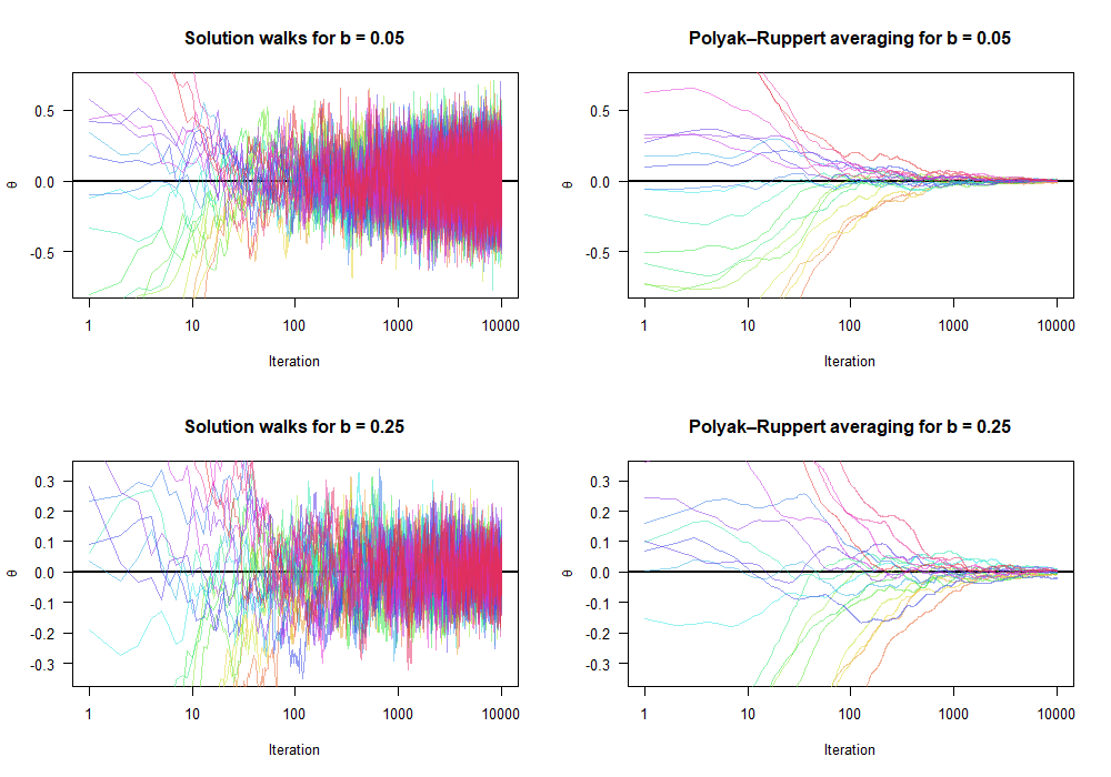
To add to @whuber's excellent answer, and to further address OP's question "How to make the RM perform better?", the condition presented where b=0.25 or less can often be a good approach if additional averaging is performed by way of Cesàro summation. Specifically, Polyak–Ruppert averaging can be used to construct rolling estimates of the $\theta$ root of the form $$\bar{\theta}_n=\frac{1}{n}\sum_{i=1}^{n-1}\theta_i$$ given the much larger steps, where $a$ must necessarily be smaller than 1 in order for the rolling average to converge correctly. One of the main benefits of Polyak–Ruppert averaging is that it is often easier to automate due to its robustness rather than tweaking the a and b parameters because a just needs to be small enough such that the iterations randomly sample the area around the target root. The figures below demonstrate this phenomenon with $b=.05$ and $b=0.25$. Of course, averaging over the independent Polyak–Ruppert averages is also a useful strategy if the independent search trajectory information is available.

Finally, below is the modification to @whuber's code for b=0.25 and the much smaller b=.05, though now with the Polyak-Ruppert averaging.

f <- function(x) {
    1/(1 + exp(-x/2)) - 1/2 + rnorm(length(x), sd=0.1)
}
#
# Specify the study parameters.
#
set.seed(17)
iterations <- seq_len(1e4)    # Specify the number of iterations
burn.period <- 1e2            # Skip these initial results when scaling the plots
replicates <- 20              # Specify how many starting values to use
bs <- c(.05, 0.25)      # Specify which `b` values to explore
as <- sort(rt(replicates, 2)) # Draw the starting values randomly
#
# Perform the study.
#
par(mfrow=c(2,2)) 
colors <- hsv(seq_along(as)/length(as), .8, .9, .5)
#
# Find the solutions for each starting value `a`.
#

for(b in bs){

    lambda <- iterations^(-b)
    solutions <- sapply(as, function(a) {
        Reduce(function(y, lambda) y - lambda * f(y), lambda, a, accumulate=TRUE)
    })
    #
    # Prepare to plot all the trajectories.
    #
    r <- range(solutions[-seq_len(burn.period), ])
    plot(range(iterations), r,
         log="x", type="n", xlab="Iteration", ylab=expression(theta), las=1,
         main=paste("Solution walks for b =", b))
    abline(h=0, lwd=2)
    #
    # Plot the trajectories.
    #
    sapply(seq_len(ncol(solutions)), function(j) {
        theta <- solutions[-1, j]
        lines(iterations, theta, cex=3/4, col=colors[j])
    })
    
    
    plot(range(iterations), r,
         log="x", type="n", xlab="Iteration", ylab=expression(theta), las=1,
         main=paste("Polyak–Ruppert averaging for b =", b))
    abline(h=0, lwd=2)
    
    sapply(seq_len(ncol(solutions)), function(j) {
        theta <- solutions[-1, j]
        thetaPR <- sapply(2L:nrow(solutions), \(i) sum(theta[1L:i]) / (i+1))
        lines(iterations, thetaPR, cex=3/4, col=colors[j])
    })
}
par(mfrow=c(1,1))