1. UNNECESSARY PROBABILITIES.
The next two sections of this note analyze the "guess which is larger" and "two envelope" problems using standard tools of decision theory (2). This approach, although straightforward, appears to be new. In particular, it identifies a set of decision procedures for the two envelope problem that are demonstrably superior to the “always switch” or “never switch” procedures.
Section 2 introduces (standard) terminology, concepts, and notation. It analyzes all possible decision procedures for the "guess which is larger problem." Readers familiar with this material might like to skip this section. Section 3 applies a similar analysis to the two envelope problem. Section 4, the conclusions, summarizes the key points.
All published analyses of these puzzles assume there is a probability distribution governing the possible states of nature. This assumption, however, is not part of the puzzle statements. The key idea to these analyses is that dropping this (unwarranted) assumption leads to a simple resolution of the apparent paradoxes in these puzzles.
2. THE “GUESS WHICH IS LARGER” PROBLEM.
An experimenter is told that different real numbers $x_1$ and $x_2$ are written on two slips of paper. She looks at the number on a randomly chosen slip. Based only on this one observation, she must decide whether it is the smaller or larger of the two numbers.
Simple but open-ended problems like this about probability are notorious for being confusing and counter-intuitive. In particular, there are at least three distinct ways in which probability enters the picture. To clarify this, let's adopt a formal experimental point of view (2).
Begin by specifying a loss function. Our goal will be to minimize its expectation, in a sense to be defined below. A good choice is to make the loss equal to $1$ when the experimenter guesses correctly and $0$ otherwise. The expectation of this loss function is the probability of guessing incorrectly. In general, by assigning various penalties to wrong guesses, a loss function captures the objective of guessing correctly. To be sure, adopting a loss function is as arbitrary as assuming a prior probability distribution on $x_1$ and $x_2$, but it is more natural and fundamental. When we are faced with making a decision, we naturally consider the consequences of being right or wrong. If there are no consequences either way, then why care? We implicitly undertake considerations of potential loss whenever we make a (rational) decision and so we benefit from an explicit consideration of loss, whereas the use of probability to describe the possible values on the slips of paper is unnecessary, artificial, and-—as we shall see—-can prevent us from obtaining useful solutions.
Decision theory models observational results and our analysis of them. It uses three additional mathematical objects: a sample space, a set of “states of nature,” and a decision procedure.
The sample space $S$ consists of all possible observations; here it can be identified with $\mathbb{R}$ (the set of real numbers).
The states of nature $\Omega$ are the possible probability distributions governing the experimental outcome. (This is the first sense in which we may talk about the “probability” of an event.) In the “guess which is larger” problem, these are the discrete distributions taking values at distinct real numbers $x_1$ and $x_2$ with equal probabilities of $\frac{1}{2}$ at each value. $\Omega$ can be parameterized by $\{\omega = (x_1, x_2) \in \mathbb{R}\times\mathbb{R}\ |\ x_1 \gt x_2\}.$
The decision space is the binary set $\Delta = \{\text{smaller}, \text{larger}\}$ of possible decisions.
In these terms, the loss function is a real-valued function defined on $\Omega \times \Delta$. It tells us how “bad” a decision is (the second argument) compared to reality (the first argument).
The most general decision procedure $\delta$ available to the experimenter is a randomized one: its value for any experimental outcome is a probability distribution on $\Delta$. That is, the decision to make upon observing outcome $x$ is not necessarily definite, but rather is to be chosen randomly according to a distribution $\delta(x)$. (This is the second way in which probability may be involved.)
When $\Delta$ has just two elements, any randomized procedure can be identified by the probability it assigns to a prespecified decision, which to be concrete we take to be “larger.”

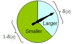
A physical spinner implements such a binary randomized procedure: the freely-spinning pointer will come to stop in the upper area, corresponding to one decision in $\Delta$, with probability $\delta$, and otherwise will stop in the lower left area with probability $1-\delta(x)$. The spinner is completely determined by specifying the value of $\delta(x)\in[0,1]$.
Thus a decision procedure can be thought of as a function
$$\delta^\prime:S\to[0,1],$$
where
$${\Pr}_{\delta(x)}(\text{larger}) = \delta^\prime(x)\ \text{ and }\ {\Pr}_{\delta(x)}(\text{smaller})=1-\delta^\prime(x).$$
Conversely, any such function $\delta^\prime$ determines a randomized decision procedure. The randomized decisions include deterministic decisions in the special case where the range of $\delta^\prime$ lies in $\{0,1\}$.
Let us say that the cost of a decision procedure $\delta$ for an outcome $x$ is the expected loss of $\delta(x)$. The expectation is with respect to the probability distribution $\delta(x)$ on the decision space $\Delta$. Each state of nature $\omega$ (which, recall, is a Binomial probability distribution on the sample space $S$) determines the expected cost of any procedure $\delta$; this is the risk of $\delta$ for $\omega$, $\text{Risk}_\delta(\omega)$. Here, the expectation is taken with respect to the state of nature $\omega$.
Decision procedures are compared in terms of their risk functions. When the state of nature is truly unknown, $\varepsilon$ and $\delta$ are two procedures, and $\text{Risk}_\varepsilon(\omega)\ge \text{Risk}_\delta(\omega)$ for all $\omega$, then there is no sense in using procedure $\varepsilon$, because procedure $\delta$ is never any worse (and might be better in some cases). Such a procedure $\varepsilon$ is inadmissible; otherwise, it is admissible. Often many admissible procedures exist. We shall consider any of them “good” because none of them can be consistently out-performed by some other procedure.
Note that no prior distribution is introduced on $\Omega$ (a “mixed strategy for $C$” in the terminology of (1)). This is the third way in which probability may be part of the problem setting. Using it makes the present analysis more general than that of (1) and its references, while yet being simpler.
Table 1 evaluates the risk when the true state of nature is given by $\omega=(x_1, x_2).$ Recall that $x_1 \gt x_2.$
Table 1.
$$\matrix {
\text{Decision:}& & \text{Larger} & \text{Larger} & \text{Smaller} & \text{Smaller}\\
\text{Outcome} & \text{Probability} & \text{Probability} & \text{Loss} & \text{Probability} & \text{Loss} & \text{Cost} \\
x_1 & 1/2 & \delta^\prime(x_1) & 0 & 1 - \delta^\prime(x_1) & 1 & 1 - \delta^\prime(x_1) \\
x_2 & 1/2 & \delta^\prime(x_2) & 1 & 1 - \delta^\prime(x_2) & 0 & 1 - \delta^\prime(x_2)
}$$
$$\text{Risk}(x_1,x_2):\ (1 - \delta^\prime(x_1) + \delta^\prime(x_2))/2.$$
In these terms the “guess which is larger” problem becomes
Given you know nothing about $x_1$ and $x_2$, except that they are distinct, can you find a decision procedure $\delta$ for which the risk $[1 – \delta^\prime(\max(x_1, x_2)) + \delta^\prime(\min(x_1, x_2))]/2$ is surely less than $\frac{1}{2}$?
This statement is equivalent to requiring $\delta^\prime(x)\gt \delta^\prime(y)$ whenever $x \gt y.$ Whence, it is necessary and sufficient for the experimenter's decision procedure to be specified by some strictly increasing function $\delta^\prime: S\to [0, 1].$ This set of procedures includes, but is larger than, all the “mixed strategies $Q$” of 1. There are lots of randomized decision procedures that are better than any unrandomized procedure!
3. THE “TWO ENVELOPE” PROBLEM.
It is encouraging that this straightforward analysis disclosed a large set of solutions to the “guess which is larger” problem, including good ones that have not been identified before. Let us see what the same approach can reveal about the other problem before us, the “two envelope” problem (or “box problem,” as it is sometimes called). This concerns a game played by randomly selecting one of two envelopes, one of which is known to have twice as much money in it as the other. After opening the envelope and observing the amount $x$ of money in it, the player decides whether to keep the money in the unopened envelope (to “switch”) or to keep the money in the opened envelope. One would think that switching and not switching would be equally acceptable strategies, because the player is equally uncertain as to which envelope contains the larger amount. The paradox is that switching seems to be the superior option, because it offers “equally probable” alternatives between payoffs of $2x$ and $x/2,$ whose expected value of $5x/4$ exceeds the value in the opened envelope. Note that both these strategies are deterministic and constant.
In this situation, we may formally write
$$\eqalign{
S &= \{ x\in \mathbb{R}\ |\ x \gt 0\}, \\
\Omega &= \{\text{Discrete distributions supported on }\{\omega, 2\omega\}\ |\ \omega \gt 0 \text{ and }\Pr(\omega) = \frac{1}{2}\}, \text{and}\\
\Delta &= \{\text{Switch}, \text{Do not switch}\}.
}$$
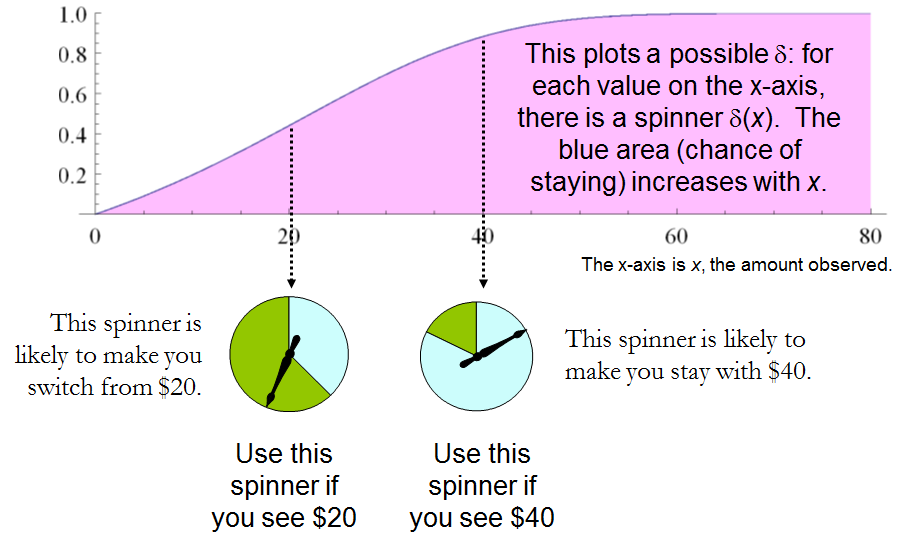
As before, any decision procedure $\delta$ can be considered a function from $S$ to $[0, 1],$ this time by associating it with the probability of not switching, which again can be written $\delta^\prime(x)$. The probability of switching must of course be the complementary value $1–\delta^\prime(x).$
The loss, shown in Table 2, is the negative of the game's payoff. It is a function of the true state of nature $\omega$, the outcome $x$ (which can be either $\omega$ or $2\omega$), and the decision, which depends on the outcome.
Table 2.
$$\matrix{
& \text{Loss}&\text{Loss} &\\
\text{Outcome}(x) & \text{Switch} & \text{Do not switch} & \text{Cost}\\
\omega & -2\omega & -\omega & -\omega[2(1-\delta^\prime(\omega)) + \delta^\prime(\omega)]\\
2\omega & -\omega & -2\omega & -\omega[1 - \delta^\prime(2\omega) + 2\delta^\prime(2\omega)]
}$$
In addition to displaying the loss function, Table 2 also computes the cost of an arbitrary decision procedure $\delta$. Because the game produces the two outcomes with equal probabilities of $\frac{1}{2}$, the risk when $\omega$ is the true state of nature is
$$\eqalign{
\text{Risk}_\delta(\omega) &=-\omega[2(1-\delta^\prime(\omega)) + \delta^\prime(\omega)]/2 + -\omega[1 - \delta^\prime(2\omega) + 2\delta^\prime(2\omega)]/2 \\
&= (-\omega/2)[3 + \delta^\prime(2\omega) - \delta^\prime(\omega)].
}$$
A constant procedure, which means always switching ($\delta^\prime(x)=0$) or always standing pat ($\delta^\prime(x)=1$), will have risk $-3\omega/2$. Any strictly increasing function, or more generally, any function $\delta^\prime$ with range in $[0, 1]$ for which $\delta^\prime(2x) \gt \delta^\prime(x)$ for all positive real $x,$ determines a procedure $\delta$ having a risk function that is always strictly less than $-3\omega/2$ and thus is superior to either constant procedure, regardless of the true state of nature $\omega$! The constant procedures therefore are inadmissible because there exist procedures with risks that are sometimes lower, and never higher, regardless of the state of nature.

Comparing this to the preceding solution of the “guess which is larger” problem shows the close connection between the two. In both cases, an appropriately chosen randomized procedure is demonstrably superior to the “obvious” constant strategies.
These randomized strategies have some notable properties:
There are no bad situations for the randomized strategies: no matter how the amount of money in the envelope is chosen, in the long run these strategies will be no worse than a constant strategy.
No randomized strategy with limiting values of $0$ and $1$ dominates any of the others: if the expectation for $\delta$ when $(\omega, 2\omega)$ is in the envelopes exceeds the expectation for $\varepsilon$, then there exists some other possible state with $(\eta, 2\eta)$ in the envelopes and the expectation of $\varepsilon$ exceeds that of $\delta$ .
The $\delta$ strategies include, as special cases, strategies equivalent to many of the Bayesian strategies. Any strategy that says “switch if $x$ is less than some threshold $T$ and stay otherwise” corresponds to $\delta(x)=1$ when $x \ge T, \delta(x) = 0$ otherwise.
What, then, is the fallacy in the argument that favors always switching? It lies in the implicit assumption that there is any probability distribution at all for the alternatives. Specifically, having observed $x$ in the opened envelope, the intuitive argument for switching is based on the conditional probabilities Prob(Amount in unopened envelope | $x$ was observed), which are probabilities defined on the set of underlying states of nature. But these are not computable from the data. The decision-theoretic framework does not require a probability distribution on $\Omega$ in order to solve the problem, nor does the problem specify one.
This result differs from the ones obtained by (1) and its references in a subtle but important way. The other solutions all assume (even though it is irrelevant) there is a prior probability distribution on $\Omega$ and then show, essentially, that it must be uniform over $S.$ That, in turn, is impossible. However, the solutions to the two-envelope problem given here do not arise as the best decision procedures for some given prior distribution and thereby are overlooked by such an analysis. In the present treatment, it simply does not matter whether a prior probability distribution can exist or not. We might characterize this as a contrast between being uncertain what the envelopes contain (as described by a prior distribution) and being completely ignorant of their contents (so that no prior distribution is relevant).
4. CONCLUSIONS.
In the “guess which is larger” problem, a good procedure is to decide randomly that the observed value is the larger of the two, with a probability that increases as the observed value increases. There is no single best procedure. In the “two envelope” problem, a good procedure is again to decide randomly that the observed amount of money is worth keeping (that is, that it is the larger of the two), with a probability that increases as the observed value increases. Again there is no single best procedure. In both cases, if many players used such a procedure and independently played games for a given $\omega$, then (regardless of the value of $\omega$) on the whole they would win more than they lose, because their decision procedures favor selecting the larger amounts.
In both problems, making an additional assumption-—a prior distribution on the states of nature—-that is not part of the problem gives rise to an apparent paradox. By focusing on what is specified in each problem, this assumption is altogether avoided (tempting as it may be to make), allowing the paradoxes to disappear and straightforward solutions to emerge.
REFERENCES
(1) D. Samet, I. Samet, and D. Schmeidler, One Observation behind Two-Envelope Puzzles. American Mathematical Monthly 111 (April 2004) 347-351.
(2) J. Kiefer, Introduction to Statistical Inference. Springer-Verlag, New York, 1987.


sum(p(X) * (1/2X*f(X) + 2X(1-f(X)) ) = X, where f(X) is the likelihood of the first envelope being larger, given any particular X. $\endgroup$