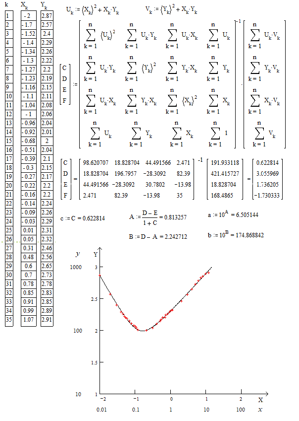
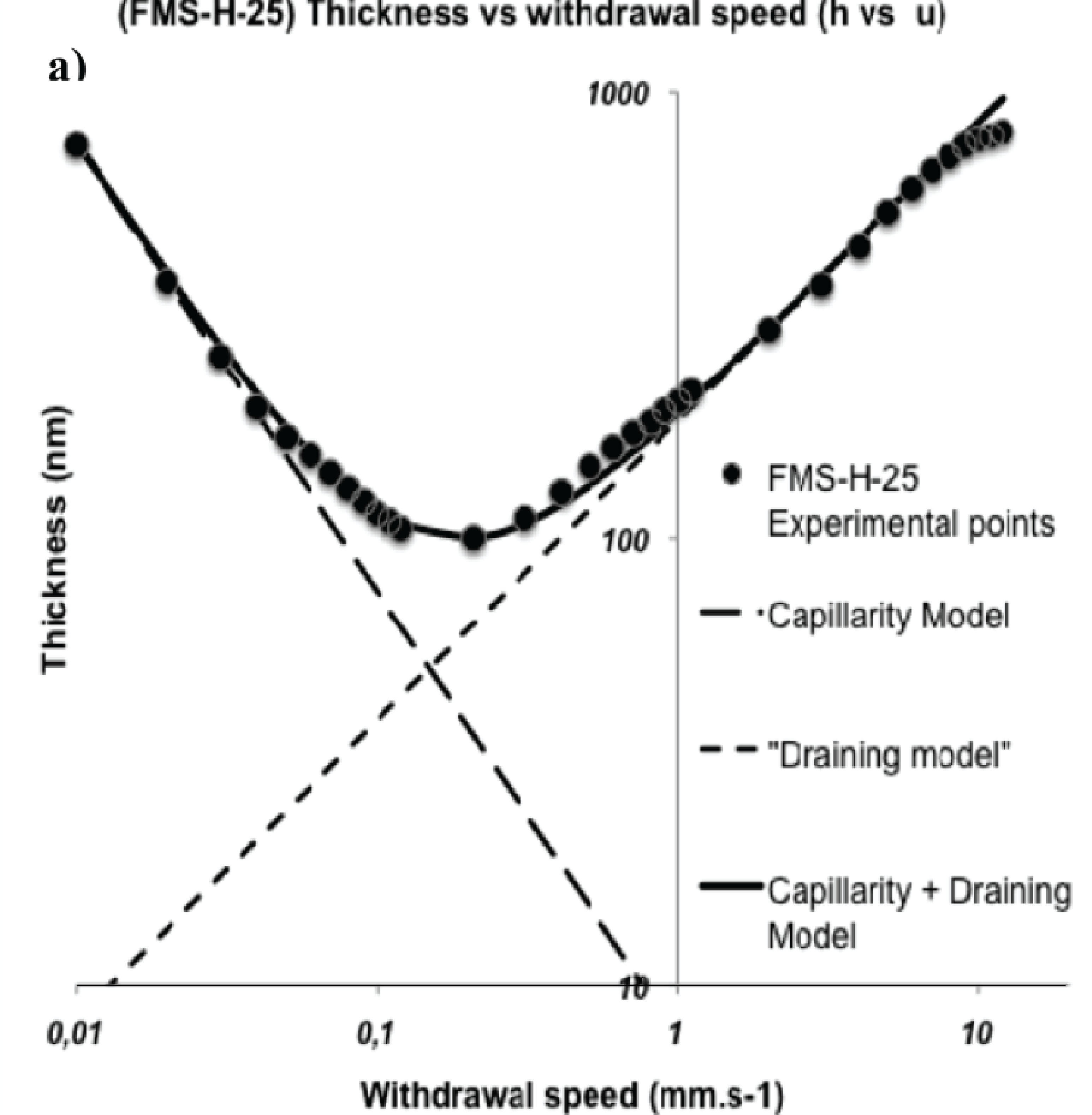
The shape of the curve looks like an hyperbola. So, we can try to fit an hyperbola to the data.
But this is probably not the best choice. I agree with the whuber's comment: A better choice of model should be derived from physical considerations.
The numerical data provided in the question apparently doesn't match to the figure. Since it is better to have more points for the example of calculus, I used the figure to generate the data below. Of course this is not very accurate due to the uncertain scanning of the pixels of the graph.
Notations :
The coordinates of the points on the graph are noted $(X_1,Y_1),(X_2,Y_2) ,..., (X_k,Y_k) ,..., (X_n,Y_n)$
Since the scales are logarithmic they correspond to the "experimental" values :
$$(x_1,y_1),(x_2,y_2) ,..., (x_k,y_k) ,...,(x_n,y_n) \quad \text{with}\quad \begin{cases} X_k=\log_{10}(x_k)\\ Y_k=\log_{10}(y_k)\end{cases}$$
Asymptotically we want $\begin{cases}
y=\frac{a}{x}\\
y=bx^c
\end{cases}\quad\implies\quad\begin{cases}
Y=A-X\\
Y=B+cX
\end{cases}$
Equation of the asymptotes : $\big(Y-(A-X)\big)\big(Y-(B+cX)\big)=0$
Equation of the hyperbola : $\big(Y-(A-X)\big)\big(Y-(B+cX)\big)=G$
$G$ is a constant to be optimiezed to fit the hyperbola to the data.
Equation of the hyperbola :
$$Y^2+(1-c)XY-cX^2-(A+B)Y+(Ac-B)X+AB-G=0$$
The optimized coefficients can be computed thanks to linear regression :
$$Y^2+XY= c(X^2+XY)+(A+B)Y+(B-Ac)X-(AB+G)$$
$$V=cU+DY+EX+F \qquad\begin{cases}
V=Y^2+XY\\
U=X^2+XY\\
D=A+B\\
E=B-Ac\\
F=-(AB+G)
\end{cases}$$
The linear regression gives $c, D,E,F\quad$ then $\quad\begin{cases}
A=\frac{D-E}{1+c}\\
B=D-A\\
\end{cases}\quad\text{and}\quad\begin{cases}
a=10^{A}\\
b=10^{B}\end{cases}$

The equation of the fitted curve comes from solving for $Y$ the next equation :
$$Y^2+(1-c)XY-cX^2-(A+B)Y+EX-F=0$$
$$Y=\frac{1}{2}\left((c-1)X+A+B+\sqrt{((c-1)X+A+B)^2+4(cX^2+EX+F}\right)$$


