GLM negative binomial - what to do when one category has only zeros?

Question

I have camera trap data for four different management types (A,B,C,D). I want to know whether there is an effect of these management types on the abundance of different mammalian herbivore species.

For some of the species, there are only zeros in one type of management, which complicates the analysis.

What do I do? I know I could do a Bayesian approach but before I go into that, I would like to know if there's a work-around that allows me to do this analysis using a frequentist approach.

The data for zebras:

    counts <- (c(67, 194, 155, 135, 146, 257, 114, 134, 111, 87, 
               62, 67, 85, 89, 63, 86, 97, 44, 0, 0, 0, 0, 0, 0))
    management <- rep(LETTERS[1:4], each = 6)

The model:

     library(MASS)
     model <- glm.nb(counts ~ management)
     summary(model)

The output shows a huge standard error for group D, that only had 0s:

    Call:
    glm.nb(formula = counts ~ management, init.theta = 
       11.27380856, 
        link = log)
    
    Deviance Residuals: 
         Min        1Q    Median        3Q       Max  
    -2.42149  -0.35526  -0.00006   0.45934   1.70106  
    
    Coefficients:
                 Estimate Std. Error z value Pr(>|z|)    
    (Intercept)    5.0689     0.1258  40.286  < 2e-16 ***
    managementB   -0.5063     0.1799  -2.815  0.00488 ** 
    managementC   -0.7208     0.1810  -3.982 6.84e-05 ***
    managementD  -25.3715  6344.9393  -0.004  0.99681    
    ---
    Signif. codes:  0 ‘***’ 0.001 ‘**’ 0.01 ‘*’ 0.05 ‘.’ 0.1 ‘ ’ 1
    
    (Dispersion parameter for Negative Binomial(11.2738) family taken to be 1)
    
        Null deviance: 339.360  on 23  degrees of freedom
    Residual deviance:  18.139  on 20  degrees of freedom
    AIC: 185.92
    
    Number of Fisher Scoring iterations: 1
    
    
                  Theta:  11.27 
              Std. Err.:  4.11 
    
     2 x log-likelihood:  -175.918 

It can also not show me any differences between 'D' and all the other groups. pairwise comparison:

    library(multcomp)
    contrasts <- c(
      "A - B = 0",
      "A - C = 0",
      "A - D = 0",
      "B - C = 0",
      "B - D = 0",
      "C - D = 0")
    
    H <- glht(model, linfct = mcp(management = contrasts))
    summary(H)

    Simultaneous Tests for General Linear Hypotheses
    
    Multiple Comparisons of Means: User-defined Contrasts
       
    Fit: glm.nb(formula = counts ~ management, init.theta = 
          11.27380856, 
        link = log)
    
    Linear Hypotheses:
                Estimate Std. Error z value Pr(>|z|)    
    A - B == 0    0.5063     0.1799   2.815 0.018355 *  
    A - C == 0    0.7208     0.1810   3.982 0.000271 ***
    A - D == 0   25.3715  6344.9393   0.004 1.000000    
    B - C == 0    0.2145     0.1829   1.173 0.597425    
    B - D == 0   24.8652  6344.9393   0.004 1.000000    
    C - D == 0   24.6507  6344.9393   0.004 1.000000    
    ---
    Signif. codes:  0 ‘***’ 0.001 ‘**’ 0.01 ‘*’ 0.05 ‘.’ 0.1 ‘ ’ 1
    (Adjusted p values reported -- single-step method)

Answer 1

Adding to the other answers with some experimental calculations. The large standard error for managementD is caused by small sample size. The standard error you've got is based on an approximation, based on the loglikelihood function being approximately quadratic, which it is not. We can try to get a confidence interval by profiling, but the R profile function do not work with glm.nb, so I try a workaround using the package bbmle:

counts <- (c(67, 194, 155, 135, 146, 257, 114, 134, 111, 87, 
               62, 67, 85, 89, 63, 86, 97, 44, 0, 0, 0, 0, 0, 0))
management <- rep(LETTERS[1:4], each = 6)

mydf <- data.frame(counts, management)

model.bbmle <- mle2(counts ~ dnbinom(mu=exp(logmu), size=exp(logtheta)),
                    method= "BFGS", parameters=list(logmu ~ 0 +  
                       management),
                    data=mydf, start=list(logmu=0, 
                      logtheta=2.42),
                    control=list(trace=1)  )

summary(model.bbmle)
Maximum likelihood estimation

Call:
mle2(minuslogl = counts ~ dnbinom(mu = exp(logmu), size = exp(logtheta)), 
    start = list(logmu = 0, logtheta = 2.42), method = "BFGS", 
    data = mydf, parameters = list(logmu ~ 0 + management), control = list(trace = 1))

Coefficients:
                   Estimate Std. Error z value     Pr(z)    
logmu.managementA   5.06898    0.12585 40.2783 < 2.2e-16 ***
logmu.managementB   4.56265    0.12856 35.4897 < 2.2e-16 ***
logmu.managementC   4.34811    0.13017 33.4038 < 2.2e-16 ***
logmu.managementD -11.55880  132.09516 -0.0875    0.9303    
logtheta            2.42213    0.36435  6.6478 2.976e-11 ***
---
Signif. codes:  0 ‘***’ 0.001 ‘**’ 0.01 ‘*’ 0.05 ‘.’ 0.1 ‘ ’ 1

-2 log L: 175.9181 

The fit is comparable to yours with glm.nb, the maximized loglikelihood is equal, (note the changed parametrization), the standard error is lower, but still huge!

Now, we can try profiling, but this do not work very well, so I will only give the code:

prof.4 <- bbmle::profile(model.bbmle, which=4, maxsteps=1000, 
                 alpha=0.005, trace=TRUE)  

 confint(prof.4)

    2.5 %    97.5 % 
       NA -89.53398 
 Warning messages:
 1: In .local(object, parm, level, ...) :
   non-monotonic spline fit to profile (logmu.managementD):  reverting from spline to linear approximation
 2: In regularize.values(x, y, ties, missing(ties), 
      na.rm = na.rm) :
  collapsing to unique 'x' values

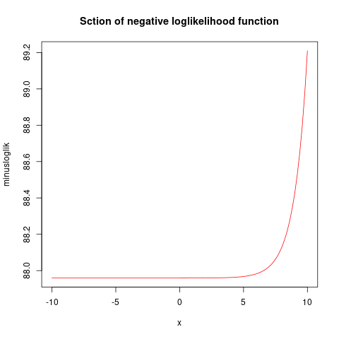
The returned interval (remember log scale!) do not make sense, and we will soon understand why. I will show a plot of a section of the loglikelihood function, along the D axes (this is not the same as profiling, since the other parameters are held fixed). This is some ugly code I do not fully understand (caused by bbmleusing S4 object system):

B <- coef(model.bbmle)

minuslogl_0 <- slot(model.bbmle, "minuslogl")

minuslogl <- function(B) do.call("minuslogl_0", namedrop(as.list(B)))

But now we can make a plot of a section of the minusloglikelihood function along the D axes, where the other parameters are held at the maxlik estimated values:

on the xaxis is the deviation of the D parameter from its maxlik value. One can see that no lower bound can be set (or, on the original scale, 0 is the lower bound), but a sharp upper bound an be set, and it will be smaller than what indicated by the standard error calculation. The code used is

delta <- 10
plot( Vectorize( function(x) minuslogl(B + c(0, 0, 0, x, 0)) ),  
     from=-delta, to=delta, ylab="minusloglik", 
     main="Section of negative loglikelihood function",
     col="red")

Answer 2

I dissent somewhat from the first answer by @dariober.

1. Adding 1 is a fudge.

2. There is no substantive reason for disbelieving zeros as recorded in the sample.

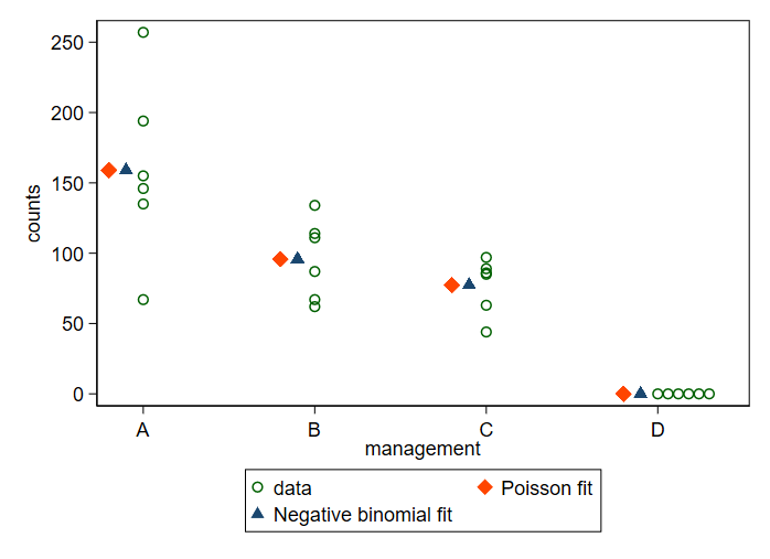
3. Most important, model fits are reasonable, the only oddity being the rather wide confidence intervals in one case. There is some robustness, as Poisson and negative binomial fits are essentially identical in fitted values. (Indeed, for this structure, all plausible models, and some not so plausible ones, essentially return group means as fitted values. The only differences are inferential small print, and if you're queasy about this you really need a bigger dataset! Easy to say....)

A graph shows it all:

For completeness, here is the Stata code I used. Naturally, the calculations are simple in any modern statistical environment.

clear 
mat counts = (67,194,155,135,146,257,114,134,111,87,62,67,85,89,63,86,97,44,0,0,0,0,0,0)
set obs 24
gen counts = counts[1, _n]
egen management = seq(), block(6)
label define management 1 A 2 B 3 C 4 D
label val management management

glm counts i.management , family(poisson)
predict poisson
glm counts i.management , family(nbinomial)
predict nbinomial 

* uncomment next if you need to install 
* ssc install stripplot 

gen management1 = management - 0.1
gen management2 = management - 0.2 

stripplot counts , over(management)  vertical stack height(0.3) legend(on order(1 "data" 2 "Poisson fit" 3 "Negative binomial fit")) yla(, ang(h)) ///
addplot(scatter poisson management2, ms(D) || scatter nbinomial management1, ms(T))

EDIT For a slightly less ad hoc method of injecting Bayes flavour than just adding 1 to all counts, I used quasi-Bayes smoothing as suggested by I.J. Good (for a self-contained account see this paper; typo fix within this paper, pp.494-495) before pushing those adjusted counts through a Poisson GLM (using robust (sandwich-Huber-Eicker-White) standard errors). The P-values make more sense while at the same time predicted means are not that different from any other fit. There will be other and arguably better ways to do this.

-------------------------------------------------------------
  management |       mean     Poisson   nbinomial  qs_Poisson
-------------+-----------------------------------------------
           A |      159.0       159.0       159.0       157.7
           B |       95.8        95.8        95.8        95.6
           C |       77.3        77.3        77.3        77.4
           D |        0.0         0.0         0.0         1.5
-------------------------------------------------------------

Answer 3

As requested by the OP in comments, I'm going to give an example in R of applying likelihood ratio test (LRT) to test differences between management groups as suggested by @GordonSmyth. I'm not sure I'm getting this right so please check it - credit goes to Gordon, faults are mine.

With LRT we check for significant differences between nested models. To apply it to this case, we need to expand the factors in management to a matrix (I guess glm does this internally anyway). Then we can drop each factor in turn and see if the simpler model differs from the full one:

library(MASS)

counts <- c(67, 194, 155, 135, 146, 257, 114, 134, 111, 87, 
            62, 67, 85, 89, 63, 86, 97, 44, 0, 0, 0, 0, 0, 0)

management <- rep(LETTERS[1:4], each = 6)

design <- model.matrix(~ management)
design
   (Intercept) managementB managementC managementD
1            1           0           0           0
2            1           0           0           0
3            1           0           0           0
4            1           0           0           0
5            1           0           0           0
6            1           0           0           0
7            1           1           0           0
8            1           1           0           0
9            1           1           0           0
10           1           1           0           0
11           1           1           0           0
12           1           1           0           0
13           1           0           1           0
14           1           0           1           0
15           1           0           1           0
16           1           0           1           0
17           1           0           1           0
18           1           0           1           0
19           1           0           0           1
20           1           0           0           1
21           1           0           0           1
22           1           0           0           1
23           1           0           0           1
24           1           0           0           1

Fit the full model, we tell glm.nb to omit the intercept since this is already encoded in the design matrix. You may want to check that this is the same using glm.nb(counts ~ management):

fit_full <- glm.nb(counts ~ 0 + design)

Now we drop group B, fit the reduced model and compare with the full one. This should be equivalent to assessing the significance of difference difference group A and group B. We get a p-value of ~0.01:

design_red <- design[, - which(colnames(design) == 'managementB')]
fit_red <-  glm.nb(counts ~ 0 + design_red)
anova(fit_full, fit_red)

Likelihood ratio tests of Negative Binomial Models

Response: counts
           Model  theta Resid. df    2 x log-lik.   Test    df LR stat. Pr(Chi)
1 0 + design_red  7.668        21          -182.4                              
2     0 + design 11.274        20          -175.9 1 vs 2     1    6.531  0.0106

We can do the same for group D:

design_red <- design[, - which(colnames(design) == 'managementD')]
fit_red <-  glm.nb(counts ~ 0 + design_red)
anova(fit_full, fit_red)
Likelihood ratio tests of Negative Binomial Models

Response: counts
           Model     theta Resid. df    2 x log-lik.   Test    df LR stat. Pr(Chi)
1 0 + design_red 829670.23        21         -1640.8                              
2     0 + design     11.27        20          -175.9 1 vs 2     1     1465       0

Unsurprisingly, the p-value for the difference between A and D is next to 0. Note that the theta parameter for the reduced model is huge and glm.nb issues warnings. I'm not sure how to interpret these but I guess it's not surprising since the intercept includes large-ish values with a string of zeros.

To test the difference between, say, B and C I would recode the full matrix to use B instead of A as intercept and proceed as above - I think there are better ways though.

Hope this helps and I got it right. However, I still think my other solution adding pseudocounts is worth considering.

Answer 4

For an explanation of why this is happening see GLM for count data with all zeroes in one category.

I know I could do a bayesian approach but before I go into that, I would like to know if there's a work-around that allows me to do this analysis using a frequentist

I think you could just add 1 to all observations and then get sensible estimates:

model <- glm.nb(counts+1 ~ management)
> summary(model)

Call:
glm.nb(formula = counts + 1 ~ management, init.theta = 
       11.87310622, link = log)

Deviance Residuals: 
    Min       1Q   Median       3Q      Max  
-2.4588  -0.3605   0.0000   0.4648   1.7339  

Coefficients:
            Estimate Std. Error z value Pr(>|z|)    
(Intercept)   5.0752     0.1228  41.330  < 2e-16 ***
managementB  -0.5022     0.1756  -2.860  0.00424 ** 
managementC  -0.7142     0.1768  -4.041 5.33e-05 ***
managementD  -5.0752     0.4425 -11.470  < 2e-16 ***
---
Signif. codes:  0 ‘***’ 0.001 ‘**’ 0.01 ‘*’ 0.05 ‘.’ 0.1 ‘ ’ 1

(Dispersion parameter for Negative Binomial(11.8731) family taken to be 1)

    Null deviance: 310.516  on 23  degrees of freedom
Residual deviance:  18.652  on 20  degrees of freedom
AIC: 198.44

Number of Fisher Scoring iterations: 1

              Theta:  11.87 
          Std. Err.:  4.23 

 2 x log-likelihood:  -188.443 

The rationale would be that zeros are not really a possible outcome and they are just a consequence of the sampling. By adding 1 you reset to a more realistic lower bound. Of course, this is acceptable if adding 1 doesn't skew the dataset too much, which doesn't seem to be the case here. I think the logic is not too dissimilar from a Bayesian approach.

---

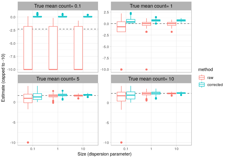
I add simulation results to illustrate the effect of adding 1 to the raw counts. Incidentally, I think this also illustrates the tradeoff between bias and variance.

I keep the counts for groups A, B, and C constant (I don't think this matters here). For group D I simulate counts from a negative binomial distribution with varying mean and size. Then I fit the glm.nb model with and without adding 1. For simplicity, I made group D to be the intercept.

Here's a summary plot of the estimates for group D, note that I reset the estimates below -10 to -10 for ease of visualization:

Horizontal lines are the true means. Each box is 500 simulations.

• When the true mean is very low (about < 1), the estimates from corrected counts noticeably overestimate the true mean (they are biased) but they are very consistent between replicates (low variance).

• Conversely, with low means, the estimates from raw counts are very unstable between replicates (high variance). After repeating the same experiment you could get considerably different results.

• When the true mean is above about 5, the effect of adding 1 starts vanishing.

I think it's up to the analyst to decide how to proceed but by gut feeling I would say that adding 1 "make sense" here. I think the issue is not so much the numerical stability of the uncorrected estimates but rather whether they are meaningful.

Code:

library(data.table)
library(ggplot2)

counts <- c(67, 194, 155, 135, 146, 257, 114, 134, 111, 87, 62, 
       67, 85, 89, 63, 86, 97, 44)
management <- rep(LETTERS[1:4], c(6, 6, 6, 6))
management <- relevel(as.factor(management), ref= 'D')

seed <- 1
dat <- list()
for(i in 1:500) {
    for(mu in c(0.1, 1, 5, 10)) {
        for(size in c(0.1, 1, 10)) {
            set.seed(seed)
            d <- data.table(
                seed= seed,
                mu= mu,
                size= size,
                counts= c(counts, rnbinom(n= sum(
                 management == 'D'), mu= mu, size= size)),
                management= management
            )
            dat[[length(dat) + 1]] <- d
            seed <- seed + 1
        }
    }
}
dat <- rbindlist(dat)

estimates <- dat[, list(raw= coef(glm.nb(counts ~   
    management))[1], corrected= coef(glm.nb(counts + 1 ~ 
    management))[1]), by= list(seed, mu, size)]
estimates <- melt(estimates, id.vars= c('seed', 'mu', 'size'), variable.name= 'method', value.name= 'estimate')

estimates[, label := sprintf('True mean count= %s', mu)]
estimates[, label := factor(label, sprintf('True mean count= %s', unique(sort(mu))))]
gg <- ggplot(data= estimates, aes(x= as.factor(size), y= 
      ifelse(estimate < -10, -10, estimate), colour= method)) +
        geom_hline(data= unique(estimates[,list(mu, label)]), 
      aes(yintercept= log(mu)), colour= 'grey30', 
      linetype= 'dashed') +
        geom_boxplot() +
        xlab('Size (dispersion parameter)') +
        ylab('Estimate (capped to -10)') +
        theme_light() +
        theme(strip.text= element_text(colour= 'black', 
        size= 12)) +
        facet_wrap(~ label, scales= 'free_y')

---

EDIT: I see quite a bit of skepticism about this solution and I'm slightly surprised about it since adding 1 to count data is not unheard of.

For example, gene expression data from sequencing technology come as count data. A very respected method of differential expression analysis is limma-voom (Gordon Smyth is a coauthor, my apologies if I'm misquoting). From the paper:

The counts are offset away from zero by 0.5 to avoid taking the log of zero, and to reduce the variability of log-cpm for low expression genes.

This is exactly what I'm proposing here.

Gene expression is never really zero and the difference between a count of 0 and a count of 1 is biologically irrelevant anyway, typically. Is it the same for the OP's case? I don't know but I suspect it is. Does it really matter whether group D has exactly 0 zebras or just 1 or 2 that went undetected in just 6 observations? If the answer is no, then adding 1 is more sensible than producing -Inf coefficients.