I'd be grateful for any help with beta-binomial (BB) regression in the gamlss package: predictions from the fitted model of "mu" values for each observation in my data seem reasonable. But the predictions for the "sigma" values do not.
exampleData <- structure(list(unit = c("F003", "F008", "F012A", "F018", "F12.SG13",
                        "F12.SG14_16", "F12_NE_L01", "F12_NW_L01", "F12_NW_L03", "F12_SE_L01",
                        "F12_SE_L02", "F12_SW_L01", "F12_SW_L03", "F12_SW_L04", "F12SE_L02A",
                        "F12SE_L03A", "F12SEL033A", "F166", "F167"),
               time = c(2.99166666666667,
                        3.06666666666667, 3.26666666666667, 2.82, 2.88571428571429, 3.13,
                        2.85652173913043, 2.91190476190476, 3.025, 2.89393939393939,
                        2.9875, 2.81176470588235, 3.11, 2.92727272727273, 2.74444444444444,
                        2.8625, 2.91, 2.94, 3.04), imported = c(58L, 20L, 13L, 10L, 24L,
                                                                25L, 85L, 62L, 46L, 49L, 22L, 96L, 22L, 17L, 11L, 57L, 81L, 15L,
                                                                6L), local = c(70L, 22L, 16L, 0L, 42L, 37L, 180L, 82L, 38L, 82L,
                                                                               30L, 129L, 9L, 11L, 0L, 187L, 157L, 11L, 0L)), class = "data.frame", row.names = c(NA,
                                                                                                                                                                  -19L))
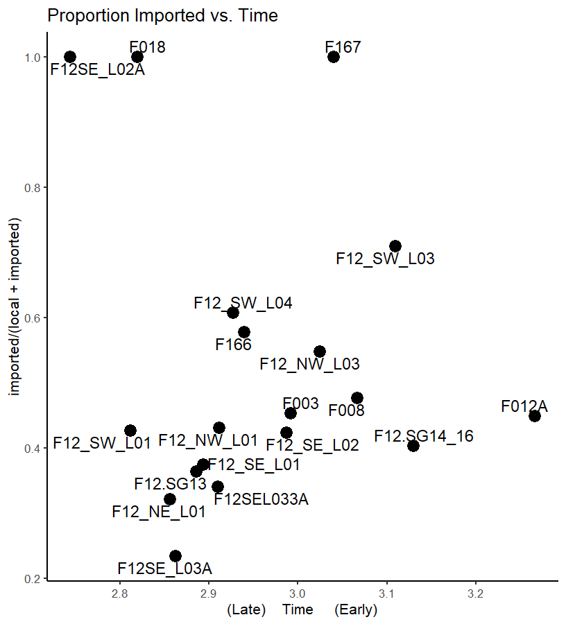
And here is a plot. The x axis is a measure of time. The y axis is the proportion of imported vs. local ceramics in 19 archaeological assemblages, computed from counts in the dataframe.
ggplot(exampleData,aes(x = time, y = imported/ (local+ imported))) +
  geom_point(shape=21,  fill='black', size=6)  +
  geom_text_repel(aes(label= unit), point.padding=1, cex=6) +
  labs(title= 'Proportion Imported vs. Time',
       x = '(Late)    Time     (Early)')
There's some theory that leads me to expect that as we go from right (early) to left (late) on the plot, we should see increased variation among assemblages in the proportion of imported ceramics. The data seem to fit that -- if you squint! But a statistical model would be nice.
The BB seems like it might work: we imagine the proportions (p) are drawn from the beta distribution, with the mean (mu) and SD (sigma) parameters changing over time. The observed counts follow binomial distributions, with parameter p drawn from a beta, with mu and sigma for the given value of time.
I try to fit this using gamlss():
library(gamlss)

model1  <- gamlss(cbind(imported, local) ~ time ,
                  sigma.formula = ~ time,
                  family=BB(mu.link = "logit", sigma.link="log"),
                  data= exampleData)

summary(model1)

GAMLSS-RS iteration 1: Global Deviance = 137.6181
GAMLSS-RS iteration 2: Global Deviance = 132.5696
GAMLSS-RS iteration 3: Global Deviance = 131.6102
GAMLSS-RS iteration 4: Global Deviance = 131.4148
GAMLSS-RS iteration 5: Global Deviance = 131.3634
GAMLSS-RS iteration 6: Global Deviance = 131.3533
GAMLSS-RS iteration 7: Global Deviance = 131.3535
Warning messages:
1: In dBB(y, mu, sigma, bd, log = TRUE) :
   values of sigma in BB less that 1e-10 are set to 1e-10
2: In dBB(y, mu, sigma, bd, log = TRUE) :
   values of sigma in BB less that 1e-10 are set to 1e-10
3: In dBB(y, mu, sigma, bd, log = TRUE) :
   values of sigma in BB less that 1e-10 are set to 1e-10
4: In dBB(y, mu, sigma, bd, log = TRUE) :
   values of sigma in BB less that 1e-10 are set to 1e-10
5: In dBB(y, mu, sigma, bd, log = TRUE) :
   values of sigma in BB less that 1e-10 are set to 1e-10
>
> summary(model1)
******************************************************************
Family:  c("BB", "Beta Binomial")

Call:  gamlss(formula = cbind(imported, local) ~ time, sigma.formula = ~time,      family = BB(mu.link = "logit", sigma.link = "log"),
    data = exampleData)

Fitting method: RS()

------------------------------------------------------------------
Mu link function:  logit
Mu Coefficients:
            Estimate Std. Error t value Pr(>|t|)
(Intercept)  -2.7035     3.4224  -0.790    0.442
time          0.8619     1.1245   0.767    0.455

------------------------------------------------------------------
Sigma link function:  log
Sigma Coefficients:
            Estimate Std. Error t value Pr(>|t|)
(Intercept)   127.37      52.35   2.433   0.0280 *
time          -45.17      18.37  -2.459   0.0266 *
---
Signif. codes:  0 ‘***’ 0.001 ‘**’ 0.01 ‘*’ 0.05 ‘.’ 0.1 ‘ ’ 1

------------------------------------------------------------------
No. of observations in the fit:  19
Degrees of Freedom for the fit:  4
      Residual Deg. of Freedom:  15
                      at cycle:  7

Global Deviance:     131.3535
            AIC:     139.3535
            SBC:     143.1313
******************************************************************
The warnings are worrisome. And it looks like there is reason to worry. When I extract the fitted values for mu, the results looks reasonable.
fitted(model1, parameter='mu' )
 [1] 0.4688241 0.4849496 0.5280128 0.4322119 0.4461619 0.4985925 0.4399530 0.4517467 0.4759850 0.4479145 0.4679299 0.4304708
[13] 0.4942830 0.4550295 0.4163059 0.4412231 0.4513401 0.4577512 0.4792108
But not for sigma:
fitted(model1, parameter='sigma' )
           1            2            3            4            5            6            7            8            9           10
3.912561e-04 1.278633e-05 1.395848e-09 9.842343e-01 4.912797e-02 7.114456e-07 1.860457e-01 1.487673e-02 8.553487e-05 3.375929e-02
          11           12           13           14           15           16           17           18           19
4.731522e-04 1.432966e+00 1.771464e-06 7.380322e-03 3.089009e+01 1.416423e-01 1.622707e-02 4.130037e-03 4.315192e-05
Note the sigma estimate for observation 15 = 30. This is impossible, since sigma must range between 0 and 1, given the parameterization of the beta that gamlss uses. And most of the other estimates seem way too small: close to 0, which is what the warnings seem to be about.
If I try to back up and simplfy by estimate and intercepts-only model, I get this:
model2  <- gamlss(cbind(imported, local) ~ 1 ,
                  sigma.formula = ~ 1,
                  family=BB(mu.link = "logit", sigma.link="log"),
                  data= exampleData)

summary(model2)
******************************************************************
Family:  c("BB", "Beta Binomial")

Call:  gamlss(formula = cbind(imported, local) ~ 1, sigma.formula = ~1,      family = BB(mu.link = "logit", sigma.link = "log"),      data = exampleData)

Fitting method: RS()

------------------------------------------------------------------
Mu link function:  logit
Mu Coefficients:
            Estimate Std. Error t value Pr(>|t|)
(Intercept) 0.002728   0.182349   0.015    0.988

------------------------------------------------------------------
Sigma link function:  log
Sigma Coefficients:
            Estimate Std. Error t value Pr(>|t|)
(Intercept)  -2.1158     0.5438  -3.891  0.00117 **
---
Signif. codes:  0 ‘***’ 0.001 ‘**’ 0.01 ‘*’ 0.05 ‘.’ 0.1 ‘ ’ 1

------------------------------------------------------------------
No. of observations in the fit:  19
Degrees of Freedom for the fit:  2
      Residual Deg. of Freedom:  17
                      at cycle:  5

Global Deviance:     147.3811
            AIC:     151.3811
            SBC:     153.2699
******************************************************************
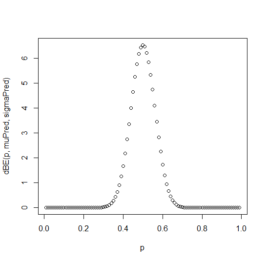
No warnings. But when I plot the beta distribution from these parameter estimates, the resulting pdf looks way to narrow to accommodate the data on the scatter plot.
muPred  <- exp(0.002728)/(1+exp( 0.002728))
sigmaPred <- exp(-2.1158)
p <- seq(.01, .99, .01)
plot(p, dBE(p, muPred, sigmaPred) )
This is my first time out with this kind of thing, so I am unsure if the problem is my understanding of the BB model, my code, a mismatch beteeen the data and the model, or something else.
Thank you for any suggestions about how to proceed.
Best, Fraser


BB. So you should probably replacedBEwithdBB. $\endgroup$