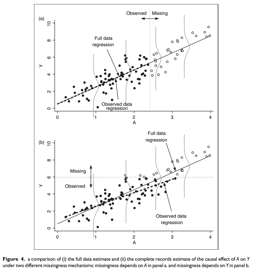
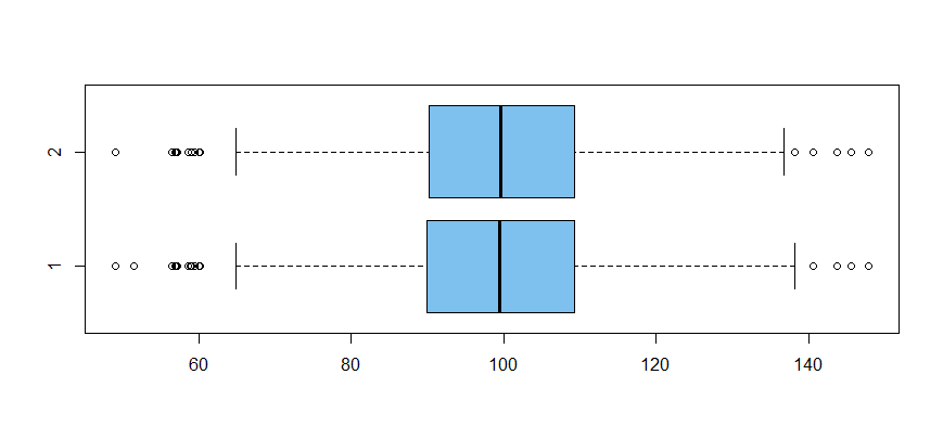
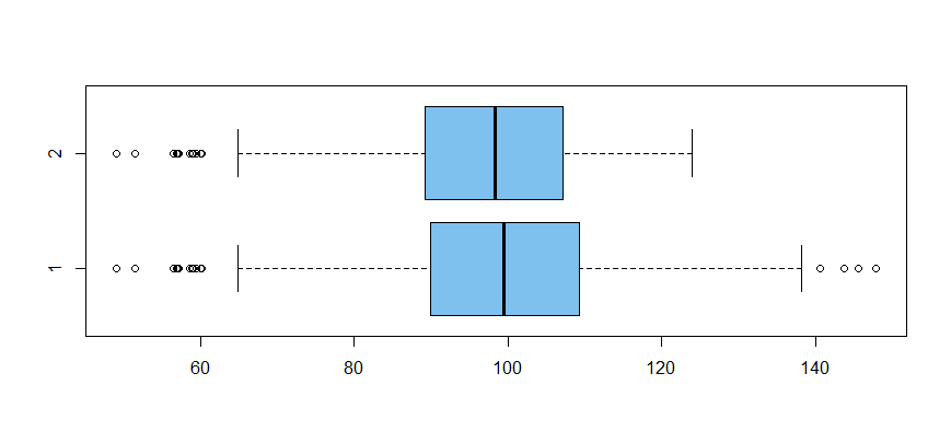
In the context of regression analysis, all of our inferences are conditional on the explanatory variables. Consequently, if the missingness is random when conditioning on these explanatory variables (which is the case for MAR) this is sufficient to ensure that estimators retain the properties they would usually have under MCAR. The basic intuition for this is that if the missingness distribution only depends on the explanatory variables then it is essentially "fixed" when we condition on these variables.
The theory of missingness is usually shown in a more generalised setting than linear regression, and its main theorems are usually established directly with respect to the likelihood function in a highly general form of analysis. A good expository paper on the concept (with theorems and proofs) is Seaman et al (2013) (version without paywall here). Below I will adapt some material from this paper to show how MAR works in the context of regression analysis. This will show that ---under the assumption of MAR--- the likelihood function for the regression parameters is proportionate to the version that "ignores" the missingness mechanism.
Setting up the problem: Consider a problem involving a set of values $(\mathbf{x}_1, \mathbf{y}_1),...,(\mathbf{x}_n, \mathbf{y}_n)$ where the conditional distribution for $\mathbf{y}|\mathbf{x}$ uses the density $f_\theta$ which depends on a parameter $\theta$. Suppose we observe this process subject to MAR with missingness indicators $\mathbf{m}_1,...,\mathbf{m}_n$ that have a conditional distribution that uses the density $g_\phi$ that depends on a parameter $\phi$. Since the sampling and missingness determine the observed outcomes, there is a mapping $H$ from any vectors of explanatory and response variables and any vector of corresponding missingness indicators to the observed vectors of explanatory and response variables.
To facilitate our analysis, let $\mathbf{x}_*$ and $\mathbf{y}_*$ denote the actual vectors of explanatory and response variables and let $\mathbf{m}_*$ denote the missingness vector that leads to the observed values. Then let $\mathbf{x}_\text{obs}$ and $\mathbf{y}_\text{obs}$ denote the observed vectors of explanatory and response variables. These latter vectors are obtained by:
$$(\mathbf{x}_\text{obs}, \mathbf{y}_\text{obs}) = H(\mathbf{x}_*, \mathbf{y}_*, \mathbf{m}_*).$$
Without loss of generality, we will suppose that there are $k = n-\sum_i m_{*i}$ observed values in the observe vectors and $n-k = \sum_i m_{*i}$ missing values that do not appear in these vectors.
Likelihood analysis: If we were to ignore the missingness mechanism in the sampling method, and just treat this as if we sampled the observed outcomes at random without any missing data, our likelihood function for inferences about $\theta$ would be:
$$L_{\mathbf{x}_\text{obs}, \mathbf{y}_\text{obs}}(\theta) = \prod_{i=1}^k f_\theta(\mathbf{y}_{\text{obs}, i}|\mathbf{x}_{\text{obs}, i}).$$
However, with the missingness mechanism the actual likelihood function is:
$$\tilde{L}_{\mathbf{x}_*, \mathbf{y}_*, \mathbf{m}_*}(\theta, \phi)
= \int \limits_{\mathscr{H}(\mathbf{x}_*, \mathbf{y}_*, \mathbf{m}_*)} \bigg( \prod_{i=1}^n f_\theta(\mathbf{y}_i|\mathbf{x}_{*i})^{1-m_{*i}} \bigg) \cdot g_\phi(\mathbf{m}_*|\mathbf{x}_*, \mathbf{y}) \ d \mathbf{y},$$
where we define the space $\mathscr{H}(\mathbf{x}_*, \mathbf{y}_*, \mathbf{m}_*)
\equiv \{ \mathbf{y} | H(\mathbf{x}_*, \mathbf{y}, \mathbf{m}_*) = H(\mathbf{x}_*, \mathbf{y}_*, \mathbf{m}_*) \}$.
Now, obviously these are very different likelihood functions. However, if missingness-at-random (MAR) holds then the distribution of the missingness vector depends on $(\mathbf{x},\mathbf{y})$ only through $\mathbf{x}$. Under this assumption we have $g_\phi(\mathbf{m}|\mathbf{x}, \mathbf{y}) = g_\phi(\mathbf{m}|\mathbf{x})$ for all $\mathbf{x},\mathbf{y},\mathbf{m}$, which then gives:
$$\begin{align}
\tilde{L}_{\mathbf{x}_*, \mathbf{y}_*, \mathbf{m}_*}(\theta, \phi)
&= \int \limits_{\mathscr{H}(\mathbf{x}_*, \mathbf{y}_*, \mathbf{m}_*)} \bigg( \prod_{i=1}^n f_\theta(\mathbf{y}_i|\mathbf{x}_{*i})^{1-m_{*i}} \bigg) \cdot g_\phi(\mathbf{m}_*|\mathbf{x}_*, \mathbf{y}) \ d \mathbf{y} \\[6pt]
&= g_\phi(\mathbf{m}_*|\mathbf{x}_*) \int \limits_{\mathscr{H}(\mathbf{x}_*, \mathbf{y}_*, \mathbf{m}_*)}\bigg( \prod_{i=1}^n f_\theta(\mathbf{y}_i|\mathbf{x}_{*i})^{1-m_{*i}} \bigg) \ d \mathbf{y} \\[6pt]
&= g_\phi(\mathbf{m}_*|\mathbf{x}_*) \int \limits_{\mathscr{H}(\mathbf{x}_*, \mathbf{y}_*, \mathbf{m}_*)}\bigg( \prod_{i=1}^k f_\theta(\mathbf{y}_{\text{obs}, i}|\mathbf{x}_{\text{obs}, i}) \bigg) \ d \mathbf{y} \\[6pt]
&= g_\phi(\mathbf{m}_*|\mathbf{x}) \cdot \bigg( \prod_{i=1}^k f_\theta(\mathbf{y}_{\text{obs}, i}|\mathbf{x}_{\text{obs}, i}) \bigg) \cdot |\mathscr{H}(\mathbf{x}_*, \mathbf{y}_*, \mathbf{m}_*)| \\[6pt]
&\propto g_\phi(\mathbf{m}_*|\mathbf{x}) \cdot \bigg( \prod_{i=1}^k f_\theta(\mathbf{y}_{\text{obs}, i}|\mathbf{x}_{\text{obs}, i}) \bigg) \\[12pt]
&= g_\phi(\mathbf{m}_*|\mathbf{x}) \cdot L_{\mathbf{x}_\text{obs}, \mathbf{y}_\text{obs}}(\theta). \\[6pt]
\end{align}$$
If we are only concerned with making inferences about $\theta$ (i.e., if $\phi$ s a nuisance parameter) then we can make use of the fact that:
$$\tilde{L}_{\mathbf{x}_*, \mathbf{y}_*, \mathbf{m}_*}(\theta, \phi) \overset{\theta}{\propto} L_{\mathbf{x}_\text{obs}, \mathbf{y}_\text{obs}}(\theta).$$
As you can see, this means that the true likelihood/profile likelihood function for the paramater $\theta$ (the one that does not ignore the missingness mechanism) is proportionate to the sipler likelihood function obtained by ignoring the missingness mechanism. If you look through the mathematics above you will see that this occurs because the equation $g_\phi(\mathbf{m}|\mathbf{x}, \mathbf{y}) = g_\phi(\mathbf{m}|\mathbf{x})$ allows us to "separate" this part from the part that depends on $\theta$ ---i.e., the MAR assumption makes the true likelihood function "seperable" with respect to the parameters $\theta$ and $\phi$.


