Using normal distribution to approximate t distribution in importance sampling

Question

The question is Exercises 6 and 7 regarding importance sampling on page 273 of Bayesian Data Analysis 3 http://www.stat.columbia.edu/~gelman/book/BDA3.pdf.

Exercise 6 approximate a normal distribution with a t distribution ($t_3$) and exercise 7 does the opposite. I do not get why the authors claim that the importance weights are well behaved when you use $t_3$ to approximate normal but they become too variable when you use normal to approximate $t_3$ because based on the output of my R code (attached below), the histogram, the effective sample size (ess) and ESS are similar in these two situations. Can someone see what the authors mean?

My second question is that exercise 7 asks to explain why the estimates of $var(\theta)$ are systematically low. I did observe this from the results. However I can not see the reason.

#BDA3  10.6
S <- 10000
sample <- rt(S,3)

w <- dnorm(sample,sd=sqrt(3))/dt(sample,3)
hist(log(w),xlim = c(-10,10))

mean <- sum(sample*w)/sum(w)

variance <- sum((sample-mean)^2*w)/sum(w)

w_tilda <- w/sum(w)
ess <- 1/(sum(w_tilda^2))
ESS <-  mean( ( w/mean(w) - 1)^2 )

mean;variance;ess;ESS

#BDA3  10.7
S <- 10000
sample <- rnorm(S,sd=sqrt(3))

w <- dt(sample,3)/dnorm(sample,sd=sqrt(3))
hist(log(w),xlim = c(-10,10))

mean <- sum(sample*w)/sum(w)

variance <- sum((sample-mean)^2*w)/sum(w)

w_tilda <- w/sum(w)
ess <- 1/(sum(w_tilda^2))
ESS <-  mean( ( w/mean(w) - 1)^2 )

mean;variance;ess;ESS
```

Answer 1

As a preliminary tip, you should always set the seed when conducting random simulations, to ensure that your work is reproducible. Also, if you want to compute the log-weights then it is best to do this directly in log-space by computing the densities in this space; this reduces numerical instability and underflow in your results. Based on correcting the above issues, here is my own (reproducible) importance sampling simulation for Exercise 6 (larger simulation only):

#Draw a sample of size S = 10000 from the approximate density
S <- 10000
set.seed(1)
SAMPLE1 <- rt(S, df = 3)

#Compute the log-weights and log-normalised-weights
LOGW1  <- dnorm(SAMPLE1, mean = 0, sd = sqrt(3), log = TRUE) - 
          dt(SAMPLE1, df = 3, log = TRUE)
LOGNW1 <- LOGW1 - matrixStats::logSumExp(LOGW1)

#Estimate the mean and variance and compute the effective sample size
NW1       <- exp(LOGNW1)
MEAN1     <- sum(NW1*SAMPLE1)
VAR1      <- sum(NW1*(SAMPLE1-MEAN1)^2)
EFF.SIZE1 <- 1/sum(NW1^2)

#Check the estimated mean and variance and the effective sample size
#True mean = 0, True variance = 3
MEAN1
[1] -0.009231501
VAR1
[1] 2.965914
EFF.SIZE1
[1] 8209.784

Now here is an importance sampling simulation for Exercise 7:

#Draw a sample of size S = 10000 from the approximate density
S <- 10000
set.seed(1)
SAMPLE2 <- rnorm(S, mean = 0, sd = sqrt(3))

#Compute the log-weights and log-normalised-weights
LOGW2  <- dt(SAMPLE2, df = 3, log = TRUE) - 
          dnorm(SAMPLE2, mean = 0, sd = sqrt(3), log = TRUE)
LOGNW2 <- LOGW2 - matrixStats::logSumExp(LOGW2)

#Estimate the mean and variance and compute the effective sample size
NW2       <- exp(LOGNW2)
MEAN2     <- sum(NW2*SAMPLE2)
VAR2      <- sum(NW2*(SAMPLE2-MEAN2)^2)
EFF.SIZE2 <- 1/sum(NW2^2)

#Check the estimated mean and variance and the effective sample size
#True mean = 0, True variance = 3
MEAN2
[1] -0.01703927
VAR2
[1] 2.129747
EFF.SIZE2
[1] 8441.093

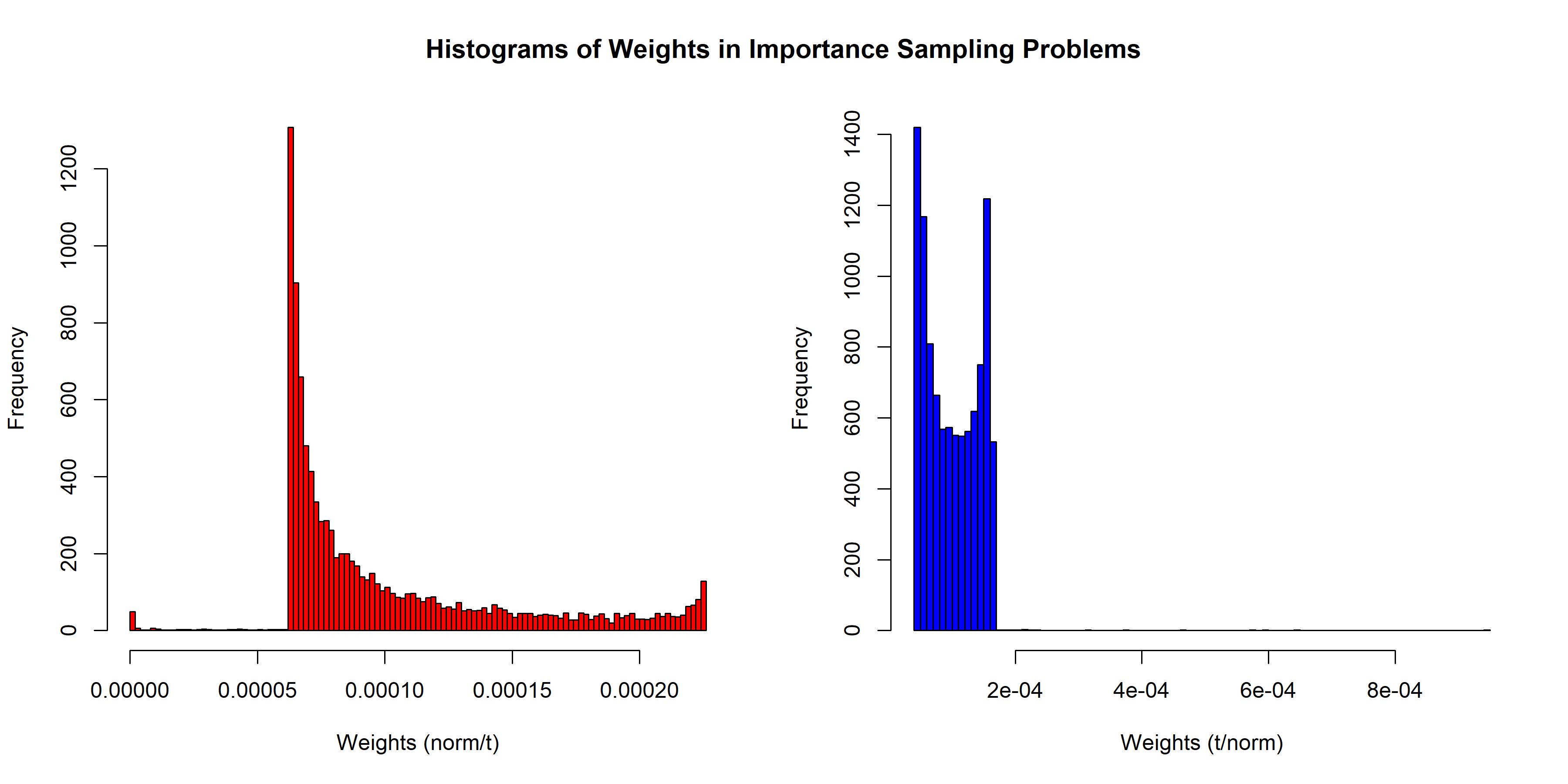
As you can see from these results, the second case results in a poor estimate of the variance. We can compare the (normalised) weights by looking at histograms:

#Setup for two plots
par(mfrow = c(1,2))

#Plot histograms of the log-normalised weights
hist(NW1, breaks = 100, col = 'red',
     main = '', xlab = 'Weights (norm/t)', ylab = 'Frequency')
hist(NW2, breaks = 100, col = 'blue',
     main = '', xlab = 'Weights (t/norm)', ylab = 'Frequency')
mtext("Histograms of Weights in Importance Sampling Problems",
      cex = 1.2, font = 2, side = 3, line = -2.4, outer = TRUE)

In assessing the two approximations, you should note the advice that the authors given regarding cases where the approximation is poor:

"The worst possible scenario occurs when the importance ratios are small with high probability but with a low probability are huge, which happens, for example, if $q$ has wide tails compared to $g$, as a function of $\theta$." (Gelman et al, p. 265)

Answer 2

Importance sampling (IS) is a method for computing expectations $E(h(\theta))$ over a target distribution $p(\theta)$ by drawing samples from an approximation $q(\theta)$: What is importance sampling?

In practice $p(\theta)$ would be a complex distribution and $q(\theta)$ would be a simpler distribution that we can sample from. In any case $p$ and $q$ would be different. (Otherwise, we would know how to sample from $p$ directly.) As we generate draws $\{\theta^s\}$ from $q$, values such that $p(\theta)/q(\theta) > 1$ are under-represented while values such that $p(\theta)/q(\theta) < 1$ are over-represented in the sample. We must correct for those differences or otherwise the importance sampling estimate would be biased.

This is where sampling weights come in: $$ \begin{aligned} w(\theta^s) = \frac{p(\theta^s)}{q(\theta^s)} \end{aligned} $$

So far the technique appears wonderfully symmetric: correct for under-representation by up-weighting and for over-representation by down-weighting. We can also show that the importance sampling estimator is consistent: it converges to $E(h(\theta))$ as the sample size $s \rightarrow \infty$.

However, (a) we never have an infinite sample and the IS estimator can be biased in a small sample. That's what happens in Exercise 7. And (b) the variance of the estimator can be infinite.

The second issue explains why large importance weights mean trouble: a few very large weights are a good indicator that the variance of the importance sampling estimator is very high or infinite. Take for example the Cauchy distribution. The Cauchy has heavy tails, so when we sample from it we get to observe very large values every now and then. At the same time, its variance is not well-defined.

And estimators with large variance are unreliable estimators.

Okay, so maybe we can look at the distribution of the sampling weights to check that their variance is not "too high". Or as the OP puts in a comment:

The authors claim that [importance sampling] does not work well if the weights are too variable, but from Ben's answer, the effective sample sizes (which is the inverse of the variance of the weights) are actually similar in these two exercises (the second case is even higher, meaning the variance of the weights in the "bad behaved" case is lower !)

Unfortunately, as Bayesian Data Analysis explains:

If the distribution has occasional very large weights, however, this estimate [ESS] is itself noisy; it can thus be taken as no more than a rough guide.

So we may not be able to use the importance weights' distribution to diagnose that the importance sampling has failed. What good is that the effective sample size is – seemingly – higher in the "badly behaved" case than in the "well behaved case" if we get a less accurate estimate of the variance? If anything, the possibility that we could end up with more confidence in a worse estimator is a cause for concern.

There are ways to address these issues. For example, Pareto-smoothed importance sampling (PSIS) models the distribution of the extreme sampling weights. (See references below.)

Learning about Pareto-smoothed importance sampling will help to:

• Understand the issues with "badly behaved" importance weights by understanding how Pareto smoothing makes importance weights more reliable.
• PSIS does come up with its own diagnostic! This is extremely useful in practice as, unlike with ESS, we would know if the estimates are not reliable.

References

A. Gelman, J. B. Carlin, H. S. Stern, D. B. Dunson, A. Vehtari, and D. B. Rubin. Bayesian Data Analysis (2013) It's available online. See Section 10.4, Importance sampling.

D. J. MacKay. Information Theory, Inference, and Learning Algorithms (2013) Also available online. See Section 29.2, Importance sampling.

R. McElreath. Statistical Rethinking: A Bayesian Course with Examples in R and STAN (2020) Free video lectures. See Section 7.4, Predicting predictive accuracy.

A. Vehtari, D. Simpson, A. Gelman, Y. Yao, and J. Gabry. Pareto smoothed importance sampling (2022) arXiv:1507.02646

All I need is time, a moment that is mine, while I'm in between [Summary of a kind of the PSIS article on Arxiv.]

Intuitive explanation of PSIS-LOO cross-validation