How to choose between ordered logit and ordered probit regression?

Question

If the dependent variable is discrete ordinal, like 0-10 then an ordered logit or ordered probit is appropriate to use. They are both similar but their interpretation are different and their error is different distributed. An ordered logit is logistically distributed and an ordered probit is normal distributed. The ordered logit have odds ratio while the ordered probit don't. Which method is used don't make a significance difference.

The above is what I read and understood from different sources. Even though I thought to plot the distribution of my data to see if it follows a logistic or normal distribution.

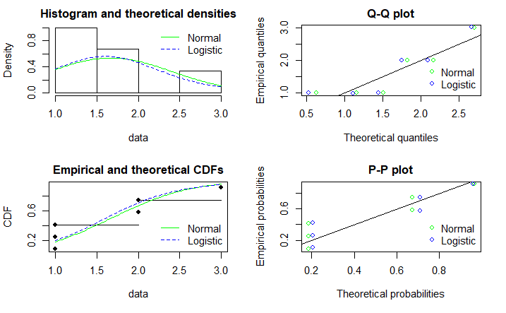
To do this I found that the plots below could be done. My question is then: is this a good way to choose between ordered logit or ordered probit?

library(effects)
library(fitdistrplus)

wvs.data = head(WVS) # data from the effects package
wvs.data
  poverty religion degree country age gender
1       1      yes     no     USA  44   male
2       2      yes     no     USA  40 female
3       1      yes     no     USA  36 female
4       3      yes    yes     USA  25 female
5       1      yes    yes     USA  39   male
6       2      yes     no     USA  80 female

wvs.data$poverty = as.numeric(wvs.data$poverty)

fit1 <- fitdist(wvs.data$poverty, "norm")
fit2 <- fitdist(wvs.data$poverty, "logis")
    
par(mfrow=c(2,2))
denscomp(list(fit1, fit2),legendtext = c("Normal", "Logistic"), 
           fitcol = c("green", "blue")) 
qqcomp(list(fit1, fit2),legendtext = c("Normal", "Logistic"), 
           fitcol = c("green", "blue")) 
cdfcomp(list(fit1, fit2),legendtext = c("Normal", "Logistic"), 
           fitcol = c("green", "blue")) 
ppcomp(list(fit1, fit2),legendtext = c("Normal", "Logistic"), 
           fitcol = c("green", "blue"))

par(mfrow=c(1, 1))
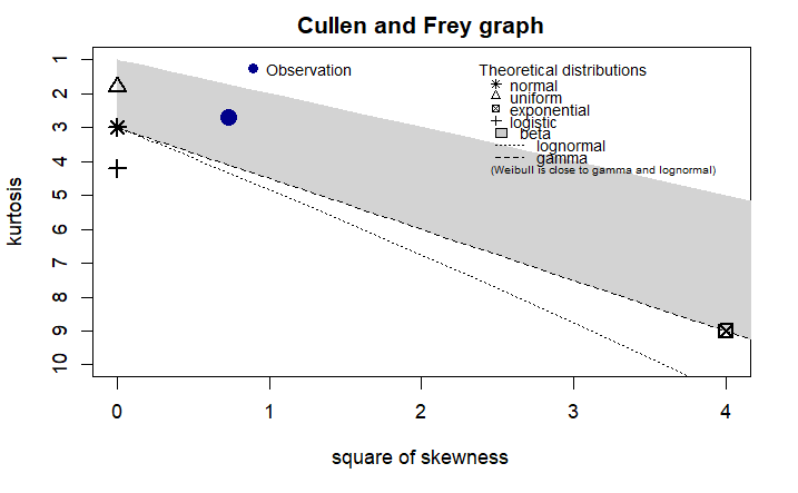
descdist(wvs.data$poverty, discrete = FALSE)
summary statistics
------
min:  1   max:  3 
median:  1.5 
mean:  1.666667 
estimated sd:  0.8164966 
estimated skewness:  0.8573214 
estimated kurtosis:  2.7 

Answer 1

It is not the outcome distribution that determines the best ordered choice model. What matters is the error term distribution in the underlying random utility or latent regression model (given the observed covariates). Unfortunately, this is not a testable assumption, and a compelling case for a particular distribution as best-in-class remains to be made. In short, looking at various characteristics of the outcome distribution while ignoring covariates is not helpful here.

The logit model has some mathematical features to recommend it, but any of these, such as computation of (effects on) odds ratios, can be replicated with the probit model under some assumptions and software-dependent inconvenience. Both models often give similar results: marginal effects, coefficients and cutpoints (except for scaling by ~1.7), z-tests, and predictions (unless the data is small or there are outliers). Both the ordered logit and probit require a parallel regression assumption, which is (sort of) testable and might lead you to a more complicated model that does alter the results.

Some criteria on how to choose between the two:

• disciplinary tradition: what will be most familiar to your audience?
• the ease of computing what you care about: what is your research question/hypothesis, or how do you plan to use the model?
• the setting for your choice problem might favor one over the other: what's in your error term?
• do both to show that results do not hinge on the choice of ex-ante sensible models and stick one in the appendix

Your question lacks detail about these considerations, so it is hard to give more practical advice on a better approach.

Answer 2

It is futile to "plot the distribution of my data to see if it follows a logistic or normal distribution."

• As Dimitriy implied, the distinction between the logit and probit models lies in the assumption of the latent, unobserved error term, not the characteristics of the observed level indicator.
• Unlike in the linear-model case, there is no residual in discrete models to estimate the error or test the error distribution. The observed outcome is a discrete event which is neither normally nor logistically distributed. In binary regression, the outcome indicator follows a Bernoulli distribution if each observation represents an individual, with a varying probability among the sample according to the specified model. If each observation represents a group, the probability of reaching an particular event count in a group follows a binomial distribution where the group size and event probability both vary among groups. In ordinal regression, the outcome indicator follows a multinomial distribution, with the event probability of each level varying among individuals and to be estimated. The fitted value, on the other hand, is an estimated event probability based on an assumption of the error-term distribution.
• Because an level indicator and the probability of a level measure totally different quantities, their difference does not represent an error term that is supposed to contrast two measurements of the same quantity. Residual quantities occurring in reference text on ordinal regression, such as Pearson and deviance residuals, are diagnostic and incomparable to residuals in linear models. See https://library.virginia.edu/data/articles/understanding-deviance-residuals.

The choice between logit and probit models is usually justified by theoretical reasons, computational convenience, and discipline convention.

• If the researcher has theoretical reasons for the error-term distribution, the choice can be argued accordingly. In a weight-loss study with the outcome measured as normal (BMI < 25), overweight (25 <= BMI < 30), or obese (BMI >= 30) for example, one may believe that the underlying BMI, which cause the ordinal categorization but is unavailable in the data, follows a normal distribution based on previous studies that have measured BMI directly. Therefore, the error term after accounting for predictor effects is also likely normally distributed, favoring the probit model. However, another can argue that the the latent error term may be logistically distributed even if the latent BMI is normally distributed, preferring a logit model. This is due to the distinction between marginal and conditional distribution. Regression assumptions are usually about the latter.
• Mathematically, logit and probit models of the same specification differ in their likelihood functions (i.e., probability mass functions) as shown at Difference between logit and probit models, just like how any type of model differs from another using the maximum likelihood estimator. The likelihood function emerges given the assumption of the distribution of the latent error term. Because the two assumed logistic and normal cumulative density functions (i.e. link functions) are extremely close in shape, as plotted at Difference between logit and probit models, logit and probit models of the same specification usually result in very similar goodness of fit, measured by log likelihoods, AIC, or BIC.
• However, it is not appropriate to overthrow one type over another solely based on goodness of fit, as their difference often happens by chance. If one must compare relative goodness of fit between a logit and a probit model for the same data, a perhaps acceptable approach is to record the differences in the log likelihoods among bootstrapped samples and to build a confidence interval or calculate a p value for the hypothesis that the logit and the probit model fit equally well. In this approach, measures like log likelihoods, AIC, or BIC are treated as individual observations. We take them over multiple samples to estimate the true parameter of goodness of fit.
• Economists seem to prefer probit models, which are deeply connected to linear models. When they need to account for random effects, instrument variables, and cross-equation correlation, an assumption of normally distributed error allows feasible model development out of a multivariate normal distribution. This is because a linear combination of normally-distributed random variables is still normally distributed, but a linear combination of logistically-distributed random variables is not logistically distributed. In engineering and health science, odds ratios prevail where authors usually present logit models, which are also faster to compute especially for multinomial outcomes.

More important than the choice between the two link functions is the assessment of linearity (i.e. location-effect specification), scale effects (i.e. variant error variance), and threshold-constant coefficients (i.e. parallel odds or parallel regression).

• These tests are all based on goodness-of-fit comparisons, giving a p value as the test result. Strategies afterwards are also stylish, as none of the tests is designed to identify the reason of violations. If the true model is y ~ x + I(x^2), whereas the specified model is y ~ x missing the squared term, test results will likely point to all of nonlinear, threshold-variant, and scale effects at the same time, suggesting different model specifications that may fit the data equally well. Selection among these specifications requires not a statistical process but subject expertise.
• Another phenomenon of which many may not be aware is that the choice between logit and probit link functions can sometimes lead to different location-effect specifications. For example, a specification of y ~ x may be sufficient in logit model, but a test of linearity could suggest y ~ x + I(x^2) when the link function is selected as probit. This usually happens only when the sample size is sufficiently large, with tens of thousands of observations to exploit the small difference in the tail distribution of logit and probit curves. The former suggests linear effects on the latent score, whereas the latter suggest parabolic effects. Likewise, one of logit and probit models may suggest scale or nominal effects while the other does not, due to fatter tails of the logistic distribution distinguishable from the normal ones in large samples.

Also more important than the choice between the two link functions are proper interpretations of the selected model.

• Assessing effect sizes solely on odds ratios can be problematic. Odds ratios can directly come from exponentiation of coefficients in logit models and be derived from predicted probabilities in probit models. Odds ratios estimated from different studies and groups are not directly comparable, unless one assumes that the unobserved error term has a constant variance across different studies and groups, which is not directly testable.
• Comparatively, comparisons based on marginal effects on probabilities are more reliable. This is typically done by calculating predicted probabilities at representative combinations of predictors, marginal effects at means, and average marginal effects across the observed predictor distribution. See the R package marginaleffects https://marginaleffects.com/files/marginaleffects_arel-bundock_greifer_heiss_jss5115.pdf for details and examples at https://marginaleffects.com/vignettes/logit.html on logit, at https://marginaleffects.com/vignettes/categorical.html on ordinal responses, and at https://marginaleffects.com/vignettes/hypothesis.html for average marginal effects. Both logit and probit models can give marginal effects on probabilities, which are easier to comprehend in common language than odds ratio. Although logit and probit models based on the same data may point to different mean structure, scale effects, or nominal effects, both models usually show very similar effects when translated onto category probabilities.
• When multiple models are plausible, model selection can introduce too much bias and subjectivity. Instead, a good practice is to present all results and discuss the implications from different perspectives. I recommend the R package ordinal to explore all these possibilities of scale and nominal effects with a variety of link functions.