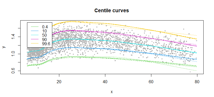
Some of the deviations you point to can be due to random variation alone. There are simple ways to test them.
When there are independent observations of a variable whose conditional distributions are continuous, then the chance that an observation is less than a quantile $q$ is -- by the very definition of quantile -- equal to $q.$ Thus, the chance the observation lies between quantiles $q$ and $q^\prime$ is $|q-q^\prime|.$
Your centiles partition the observations into six non-overlapping bins bounded by the quantiles $(0, 0.4, 10, 50, 90, 99.6, 100)/100.$ Accordingly, the likelihood (conditional on the model) of observing counts in this bins is Multinomial. Specifically, the probability of observing a count vector $(n_1,n_2,\ldots, n_6)$ (when the model is correct across the entire range of $x$ values in the data) is
$$\mathcal L(\mathbf n) = \binom{n}{n_1,n_2,\ldots,n_6} \left(\frac{0.4 - 0}{100}\right)^{n_1}\left(\frac{10 - 0.4}{100}\right)^{n_2}\cdots \left(\frac{100 - 99.6}{100}\right)^{n_6}$$
where $n = n_1 + n_2 + \cdots n_6$ is the total.
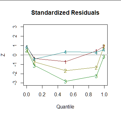
Assuming there are approximately $n=3000$ observations, the (natural) log likelihoods of these four models work out to $(-17.1, -18.5, -21.2, -16.7)$ in order. The largest likelihood of $-16.7$ identifies model (4) as having the highest likelihood. This does not mean it's a great model: to assess that, we should look at the details. A method that is easy to interpret is to plot the differences between the observed proportions $x_i$ and the proportions indicated by the centiles, $q_i,$ divided by their standard errors. The latter equal $\sqrt{q_i(1-q_i)/n}.$ Although these standardized residuals aren't truly independent, the expected counts in each bin are large enough that this makes no difference. Generally we hope most standardized residuals for any model will lie between $-2$ and $2,$ perhaps with a few of them slightly exceeding these thresholds.

Evidently models 4 and 1 have consistently near-zero residuals across the range of quantiles: they don't appreciably under- or over-estimate the conditional quantiles anywhere. Model 2 tends to have too many low counts (that is, it underestimates the middle quantiles) while Model 3 is significantly worse than any of the others.
Significance can be determined by the Likelihood Ratio (LR) test: the p-value is the tail area of a $\chi^2(1)$ distribution evaluated at twice the difference of log likelihoods. Again using $n=3000,$ I find p-values of $(0.372, 0.057, 0.003, 1.000)$ for these four models (relative to the best). Even accounting for the multiple testing, $0.003$ is so low we ought to reject model 3 as poorer than the best model. However, we shouldn't reject the other models outright: their differences could be due to chance alone.
Here is R code to produce the image. Most of it reads and formats the data and then initializes the plot. The last block of code does the calculations.
x <- scan(text = "% of cases below  0.4 centile is  0.5006258
% of cases below  10 centile is  9.803922
% of cases below  50 centile is  49.35336
% of cases below  90 centile is  90.2378
% of cases below  99.6 centile is  99.70797
% of cases below  0.4 centile is  0.458907
% of cases below  10 centile is  9.595327
% of cases below  50 centile is  48.47726
% of cases below  90 centile is  89.27826
% of cases below  99.6 centile is  99.70797
% of cases below  0.4 centile is  0.458907
% of cases below  10 centile is  9.386733
% of cases below  50 centile is  47.43429
% of cases below  90 centile is  88.77764
% of cases below  99.6 centile is  99.58281
% of cases below  0.4 centile is  0.5006258
% of cases below  10 centile is  9.762203
% of cases below  50 centile is  50.31289
% of cases below  90 centile is  90.15436
% of cases below  99.6 centile is  99.66625",
          what = c(rep(character(), 7), numeric()))

n <- 3e3
p <- c(0.4, 10, 50, 90, 99.6) / 100
x <- matrix(as.numeric(matrix(x, 8)[8,]), length(p))

q <- apply(x, 2, function(x) pbinom(round(x/100 * n), n, p))

plot(0:1,c(-3,3), type = "n", xlab = "Quantile", ylab = "Z",
     main = "Standardized Residuals")
abline(h = 0, lwd = 2, col = "gray")

sapply(1:ncol(q), function(j) {
  r <- x[,j] / 100 - p
  se <- sqrt(p * (1-p) / n)
  lines(p, r/se, col = hsv((j-1)/6, .9, .5))
  points(p, r/se, pch = as.character(j), col = hsv((j-1)/6, .9, .5))
})


