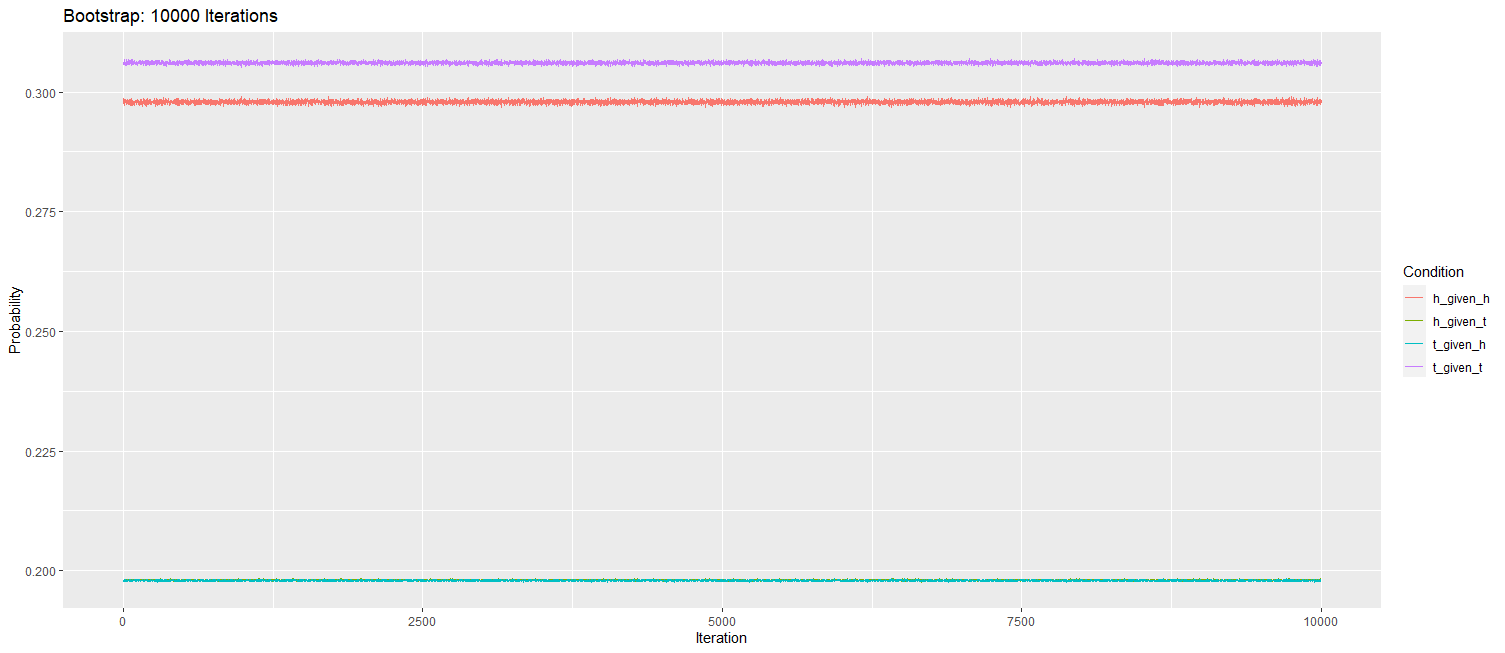
This is a problem I have been curious about for some time now.
Suppose:
- There is a coin where if it lands head then the probability of the next flip being heads is 0.6 (and if tails then the next flip being tails is also 0.6)
- There are 100 students in a class
- Each student flips this coin a random number of times
- The last flip of student_n does not influence the first flip of student_n+1 (i.e. when the next student flips the coin, the first flip has 0.5 probability of heads or tails, but the next flip for this student depends on the previous flip)
Here is some R code to represent this problem:
library(tidyverse)

set.seed(123)
ids <- 1:100
student_id <- sort(sample(ids, 100000, replace = TRUE))
coin_result <- character(1000)
coin_result[1] <- sample(c("H", "T"), 1)

for (i in 2:length(coin_result)) {
  if (student_id[i] != student_id[i-1]) {
    coin_result[i] <- sample(c("H", "T"), 1)
  } else if (coin_result[i-1] == "H") {
    coin_result[i] <- sample(c("H", "T"), 1, prob = c(0.6, 0.4))
  } else {
    coin_result[i] <- sample(c("H", "T"), 1, prob = c(0.4, 0.6))
  }
}

#tidy up
my_data <- data.frame(student_id, coin_result)
my_data <- my_data[order(my_data$student_id),]

final <- my_data %>%
    group_by(student_id) %>%
    mutate(flip_number = row_number())
The data looks something like this:
# A tibble: 6 x 3
# Groups:   student_id [1]
  student_id coin_result  flip_number
       <int> <chr>              <int>
1          1 H                      1
2          1 H                      2
3          1 H                      3
4          1 H                      4
5          1 T                      5
6          1 H                      6
My Problem: In this scenario, let's say that I do not have any prior knowledge about this coin (i.e. I only have access to the data from the students) and I think its possible that the coin might have "correlated probabilities" - particularly, I think the result of the previous flip might influence the next flip. To test this hypothesis, I can count the number of sequences observed:
final %>%
    group_by(student_id) %>%
    summarize(Sequence = str_c(coin_result, lead(coin_result)), .groups = 'drop') %>%
    filter(!is.na(Sequence)) %>%
    count(Sequence)

# A tibble: 4 x 2
  Sequence     n
  <chr>    <int>
1 HH         253
2 HT         186
3 TH         182
4 TT         279
From these results, it seems like the result of a coin flips appears to be influenced by the previous flip - however, I am interested in placing Confidence Intervals around these estimates.
I know that in general, this type of problem is characterized by a Multinomial Distribution (e.g. if the coin had more than two sides) and that there are exact formulae for Confidence Intervals based on the Multinomial Distribution. However, I am interested in learning about how to use Bootstrapping in this problem.
Right away, I can see that if the standard Bootstrapping approach is used, we will likely "interrupt" the sequence of flips - that is, we might get the $n^{\text{th}}$ flip for the $j^{\text{th}}$ student immediately followed by the $n^{\text{th}}$ flip for the $k^{\text{th}}$ student , thus invalidating the estimates produced from the Bootstrapping.
The first idea that comes to mind is to modify the Bootstrapping procedure so that the sampling process is not interrupted. For example:
- Approach 1: Randomly sample with replacement students until you have the same number of students as the original data. Using all available data for these students, calculate the probabilities and 95% Confidence Intervals. Repeat this process $k$ times
- Approach 2: Randomly sample with replacement students until you have the same number of students as the original data. For each of these students selected, randomly choose a starting point $x$ and ending point $y$ (where $y > x$), and select all available data between $x$ and $y$ for a given student. Then, calculate the probabilities and 95% Confidence Intervals. Repeat this process $k$ times.
Here is my attempt at Approach 1:
# Initialize
results <- data.frame(iteration_number = numeric(0),
                      h_given_h = numeric(0),
                      h_given_t = numeric(0),
                      t_given_h = numeric(0),
                      t_given_t = numeric(0))

# Set the number of iterations
n_iter <- 1000

# Loop
for (i in 1:n_iter) {
  # Randomly sample 100 student ids with replacement
  sampled_ids <- sample(ids, 100, replace = TRUE)

  # Select rows for sampled students
  sampled_data <- my_data[my_data$student_id %in% sampled_ids, ]

  final <- sampled_data %>%
    group_by(student_id) %>%
    mutate(flip_number = row_number())

  # Calculate conditional probabilities
  cond_prob <- final %>%
    group_by(student_id) %>%
    summarize(Sequence = str_c(coin_result, lead(coin_result)), .groups = 'drop') %>%
    filter(!is.na(Sequence)) %>%
    count(Sequence) %>%
    mutate(prob = n / sum(n))

  # Extract probabilities
  p_HH <- cond_prob$prob[cond_prob$Sequence == "HH"]
  p_HT <- cond_prob$prob[cond_prob$Sequence == "HT"]
  p_TH <- cond_prob$prob[cond_prob$Sequence == "TH"]
  p_TT <- cond_prob$prob[cond_prob$Sequence == "TT"]

  # Create a vector with the probabilities
  prob_vector <- c(p_HH, p_HT, p_TH, p_TT)
  print(prob_vector)
  # Append
  results[i, ] <- c(i, prob_vector)
}

colnames(results) <- c("iteration_number", "h_given_h", "h_given_t", "t_given_h", "t_given_t")

library(ggplot2)
results_long <- tidyr::pivot_longer(results, cols = -iteration_number, names_to = "condition", values_to = "probability")

# Plot
ggplot(results_long, aes(x = iteration_number, y = probability, color = condition)) +
  geom_line() +
  labs(x = "Iteration", y = "Probability", color = "Condition")
Then, based on these results - I can calculate the 95% Confidence Intervals based on the Quantile function:
          h_given_h_percentiles <- quantile(results$h_given_h, c(0.05, 0.95))
    h_given_t_percentiles <- quantile(results$h_given_t, c(0.05, 0.95))
    t_given_h_percentiles <- quantile(results$t_given_h, c(0.05, 0.95))
    t_given_t_percentiles <- quantile(results$t_given_t, c(0.05, 0.95))

    percentiles_results <- data.frame(condition = c("h_given_h", "h_given_t", "t_given_h", "t_given_t"),
                                 `5%` = c(h_given_h_percentiles[1], h_given_t_percentiles[1], t_given_h_percentiles[1], t_given_t_percentiles[1]),
                                 `95%` = c(h_given_h_percentiles[2], h_given_t_percentiles[2], t_given_h_percentiles[2], t_given_t_percentiles[2]))

# Calculate the mean for each column
h_given_h_mean <- mean(results$h_given_h)
h_given_t_mean <- mean(results$h_given_t)
t_given_h_mean <- mean(results$t_given_h)
t_given_t_mean <- mean(results$t_given_t)

percentiles_results$mean <- c(h_given_h_mean, h_given_t_mean, t_given_h_mean, t_given_t_mean)

  condition       X5.      X95.      mean
1 h_given_h 0.2973799 0.2984679 0.2979292
2 h_given_t 0.1978462 0.1981885 0.1980179
3 t_given_h 0.1977906 0.1981054 0.1979481
4 t_given_t 0.3056818 0.3065346 0.3061047
My Question: Can someone please tell if this approach to Bootstrapping Longitudinal/Repeated Measures data is statistically valid? Or is what I have done meaningless?
Thanks!
References:
- https://pratheepaj.github.io/bootLong/articles/bootLong.html
- https://link.springer.com/article/10.3758/s13428-019-01252-y
- Bootstrapping with repeated measurements
- https://link.springer.com/content/pdf/10.3758/BF03202577.pdf
- https://arxiv.org/abs/1809.01832
Note: I am currently finalizing the R Code for Approach 2 - if someone is interested, I can also post it.

