How to know errorbars on accuracy to nonlinear fit: $A(1-\cos(x+\phi))$ with poisson noise?

Question

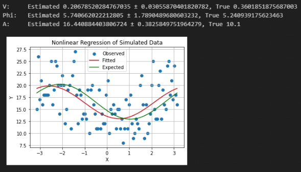
I am trying to write some code that accurately estimates the parameters for the following function:

$$ Y = A(1-V \cos(X+\phi)) $$,

where this output data is poisson distributed.

To do this, I first created a simulation of what this data would look like. Then I tried to use nonlinear regression using curve_fit in python to estimate the parameters. But I've noticed that my estimates are consistently not matched to the true value, and the true value is outside of the errorbars of the estimates given, even when I attempt a "boot-strapping" technique to estimate the errors.

For example, here you can see that it does not get the errors right.

I understand that for noisy data, such fits should be difficult, but a proper estimate should have large errorbars to reflect this.

Any ideas what is going wrong here?

Here is the code used to generate these things:

import numpy as np
import matplotlib.pyplot as plt
from scipy.optimize import curve_fit
from sklearn.utils import resample

def visibility(x, V, phi, A):
    return A*(1 - V * np.cos(x + phi))

def bootstrap_function_fit(x, y, N=5000):
    estimates = np.zeros((N, 3))
    for n in range(N):
        X_res, Y_res = resample(x, y)
        params, _ = curve_fit(visibility, X_res, Y_res, p0=guess, bounds=([0, 0, -np.inf], [1, 2*np.pi, np.inf]))
        estimates[n, :] = params
    return estimates

# True values for V and phi
V_true = np.random.uniform(0.1, 1)
phi_true = np.random.uniform(0, 2*np.pi)
A_true = 10.1

# Generate X values
X = np.linspace(-np.pi, np.pi, 100)

# Generate Y values without noise
Y_exp = visibility(X, V_true, phi_true, A_true)

# Add Poisson noise, note Y must be non-negative.
Y_obs = np.random.poisson(Y_exp + abs(Y_exp.min()) + 0.01)

# Initial guess for our parameters (V, phi, A)
guess = [0.5, np.pi, 5.0]

# Nonlinear regression: Fit the function to the data to get best fit parameters
params, params_cov = curve_fit(visibility, X, Y_obs, p0=guess, bounds=([0, 0, -np.inf], [1, 2*np.pi, np.inf]))
V_estimated, phi_estimated, A_estimated = params

# Bootstrap error estimation
estimates = bootstrap_function_fit(X, Y_obs, N=5000)

V_estimated_error = np.std(estimates[:, 0])
phi_estimated_error = np.std(estimates[:, 1])
A_estimated_error = np.std(estimates[:, 2])

# Compare estimated and true values
print(f"V:     Estimated {V_estimated} ± {V_estimated_error}, True {V_true}")
print(f"Phi:   Estimated {phi_estimated} ± {phi_estimated_error}, True {phi_true}")
print(f"A:     Estimated {A_estimated} ± {A_estimated_error}, True {A_true}")



plt.scatter(X, Y_obs, label='Observed')
plt.plot(X, visibility(X, *params), color='red', label='Fitted')
plt.plot(X, Y_exp + abs(Y_exp.min()) + 0.01, color='green', label='Expected')
plt.title('Nonlinear Regression of Simulated Data')
plt.xlabel('X')
plt.ylabel('Y')
plt.legend()
plt.grid(True)
plt.show()