Bivariate normal covering circles and ellipses

Question

I am looking at covering circles for cartesian coordinates given by independent bivariate random variables $X, Y \sim N(0, \sigma)$.

The radius of a circle that will cover proportion p of these samples is given by the Rayleigh distribution quantile function: $R(p, \sigma) = \sigma \sqrt{-2 \ln(1-p)}$.

Interestingly, if the variance in each axis is unequal – $X \sim N(0, \sigma_x), Y \sim N(0, \sigma_y)$ – then the Rayleigh quantile function gives the semi-axes of a covering ellipse: I confirmed through Monte Carlo simulation that an ellipse with $a = \sigma_x \sqrt{-2 \ln(1-p)}$ and $b = \sigma_y \sqrt{-2 \ln(1-p)}$ covers exactly proportion p of such samples.

What is a formula for a covering circle in the unequal variance case?

I found that a circle based on the mean variance $\sigma_{xy}^2=\frac{\sigma_x^2+\sigma_y^2}{2}$ is always* larger than needed to cover proportion p. I.e., a circle with radius $R(p, \sqrt{\sigma_{xy}^2})$ always covers more than p of the samples. *ETA from comment and associated graph: This is true for p < ~79%; for larger p the circle always undercovers.

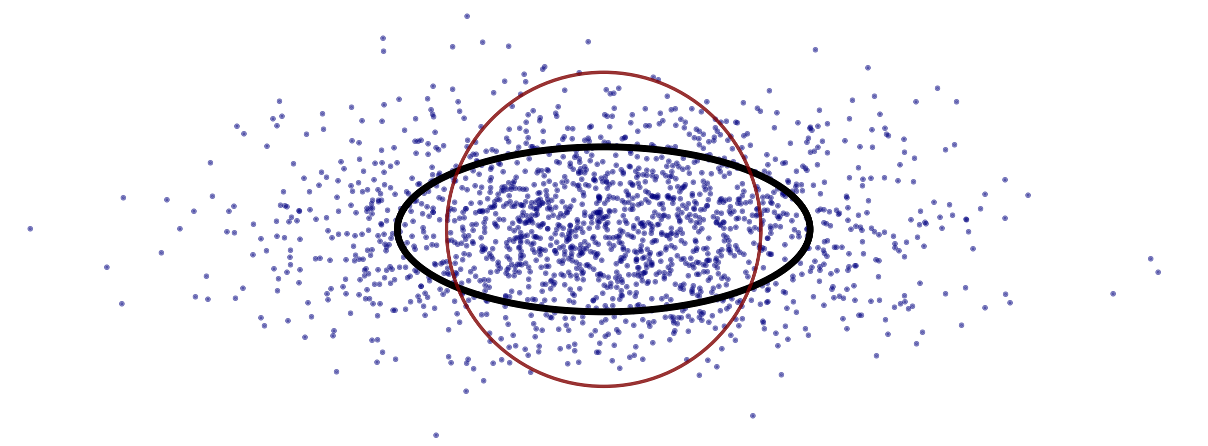
Here's an example showing the 60% covering ellipse in a scenario where $\sigma_x=2.5\sigma_y$. The red circle has radius = $\sqrt{\sigma_{xy}^2}$ and covers 65% of sample points.

(Given that the formula for the covering ellipse is so simple, I am hopeful that there is an elegant expression to circularize the unequal variance cases. I have a hunch that the normal quantile function provides information needed, and that the magic inflection point at 79% covering is exactly $\sqrt{2/\pi}$ which, i.a., is the mean of the standard half-normal. But I have minimal experience with this area of mathematics.)

Answer 1

What you want is the radius $r$ such that the cdf $P(\sqrt{X^2+Y^2}\leq r)=\alpha$ for some alpha. It is clear that $P(\sqrt{X^2+Y^2} \leq r)=P(X^2+Y^2 \leq r^2)$, and it is easier to work with the sums of squared variables.

We can think of $X^2$ and $Y^2$ as given by $X^2=Z_1\sigma_X^2$ and $Y^2=Z_2\sigma_Y^2$ where $Z_1\sim \chi^2_1$ and $Z_2\sim \chi^2_1$ are chi-squared variables with 1 degree of freedom. Given that the chi-squared is a special case of the Gamma distribution, $\chi^2_n = \mathrm{Gamma}(n/2, \frac{1}{2})$ (using the scale-rate parametrization), and using the scaling property of the gamma distribution, we have that $X^2 \sim \mathrm{Gamma}(1/2,\frac{1}{2\sigma^2_X})$ and $Y^2 \sim \mathrm{Gamma}(1/2,\frac{1}{2\sigma^2_Y})$. Thus, we need to find the distribution for the sum of two independent Gamma distributions.

This post gives an expression for the pdf of the sum of two Gamma variables, which you could use to compute the radius suitable for your alpha. Simplifying the expression, for our specific Gammas, the PDF for the sum of squares $S=X^2 + Y^2$:

$P(S) = \left\{\begin{array}{cc}\hfill \frac{e^{-S/(2\sigma_X^2)}}{2\sigma_X\sigma_Y} {}_1F_1\left[\frac{1}{2}, 1, \frac{1}{2} \left(\frac{1}{\sigma_X^2}-\frac{1}{\sigma_Y^2} \right) S \right] \hfill & ,\hfill S >0\hfill \\ {}\hfill 0 & , \hfill S \le 0 \end{array}\right.$

Ideally you'd want the cumulative probability function for your purpose, but I couldn't find such formula. We can obtain it by numerically integrating the PDF though:

import numpy as np
from scipy.special import hyp1f1
import matplotlib.pyplot as plt

# Define pdf function
def radius_squared_pdf(sigmax, sigmay, S):
    b1 = 1/(2*(sigmax**2))
    b2 = 1/(2*(sigmay**2))
    hyp1f1Res = hyp1f1(0.5, 1, (b1-b2)*S)
    pdf = (b1**(0.5)) * (b2**(0.5)) * np.exp(-S*b1) * hyp1f1Res
    return pdf

# Choose R.V. parameters
sx = 0.5
sy = 1.5
# Set parameters to integrate squared radius PDF
Smax = 20
dS = 0.001
nSteps = int((Smax-dS)/dS)
S = np.linspace(start=dS, stop=Smax, num=nSteps) # squared radius to evaluate
# Evaluate PDF
pdf = radius_squared_pdf(sx, sy, S) 
# Integrate PDF
cdf = np.cumsum(pdf*dS)

plt.plot(S, cdf)
plt.ylabel('CDF')
plt.xlabel('Squared radius')
plt.show()

# Find radius corresponding to 95% probability
alpha = 0.95
idx = np.argmin(np.abs(cdf-alpha))
r = np.sqrt(S[idx])
print(f'Radius containing {alpha*100}% of the points: {r}')

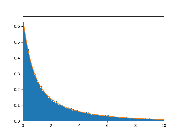
Through simulation, we can see below that the match of the analytic pdf to simulations is as we would expect (example, sx = 0.5, sy=1.5, code not shown)):

In sum, what you'd want to do is numerically integrate this formula to find the value of $r^2$ so that $P(S\leq r^2)$ equals your desired $\alpha$. Then the circle you want will have radius $r$. This is shown in the code above.