12
$\begingroup$

I just learned that a MoM estimator is not unique... What does that mean? What does being unique mean in general?

For example, if we were to find the mean using a MoM estimator for a uniform distribution, this will be $(a+b)/2$, right? Is it considered nonunique, because there are two variables?

$\endgroup$
2
  • 6
    $\begingroup$ That is not a method of moments estimator of the mean for a uniform distribution, as it uses the distribution parameters $a$ and $b$ and no data is involved. It is just a straightforward calculation of the mean. The sample mean - a function of the data - would be an MoM estimator of the mean of the uniform distribution. $\endgroup$
    – jbowman
    Commented Jan 17 at 23:08
  • 2
    $\begingroup$ To expand on jbowman's comment, the uniform distribution on $(a, b)$ has two parameters, so you will need two moments in order to solve the corresponding system of equations. As shown by Henry's answer, the resulting estimate will depend on which two moments you choose (and thus MoM is not unique). $\endgroup$
    – knrumsey
    Commented Jan 18 at 3:51

3 Answers 3

30
$\begingroup$

Let's take a different example, a random variable $X$ having a Poisson distribution with parameter $\lambda$.

  • You can say $\mathbb E[X] = \lambda$, so $\hat \lambda_1 = \frac1n\sum X$ is a method of moments estimator.

  • You can also say $\mathbb E[X^2] = \lambda+\lambda^2$, so $\hat \lambda_2 = \sqrt{\frac14+\frac1n\sum (X^2)}-\frac12$ is a different method of moments estimator.

  • You can also say $\mathbb E[X^2-X] = \lambda^2$, so $\hat \lambda_3 = \sqrt{\frac1n\sum (X^2) -\frac1n\sum X}$ is another method of moments estimator.

  • You can even take the average of these three (or two of them) and get yet another method of moments estimator, and there are infinitely more possibilities.

The second and third estimators are not good estimators: they are less natural and are biased downwards and have a higher variance than the first, but they are still estimators.

$\endgroup$
1
7
$\begingroup$

The method of moments means

that you are estimating the population parameters by selecting the parameters such that for certain specific moments the population distribution has the moments that are equivalent to the observed moments in the sample.

(What is the Method of Moments and how is it different from MLE?)


Example: for the uniform distribution example we have

$$\begin{array}{} E[X] &=& \frac{b^2-a^2}{2(b-a)} \\ E[X^2] &=& \frac{b^3-a^3}{3(b-a)} \\ E[X^3] &=& \frac{b^4-a^4}{4(b-a)} \\ E[X^4] &=& \frac{b^5-a^5}{5(b-a)} \\ \dots \\ E[X^n] &=& \frac{b^{n+1}-a^{n+1}}{(n+1)(b-a)} \\ \end{array}$$

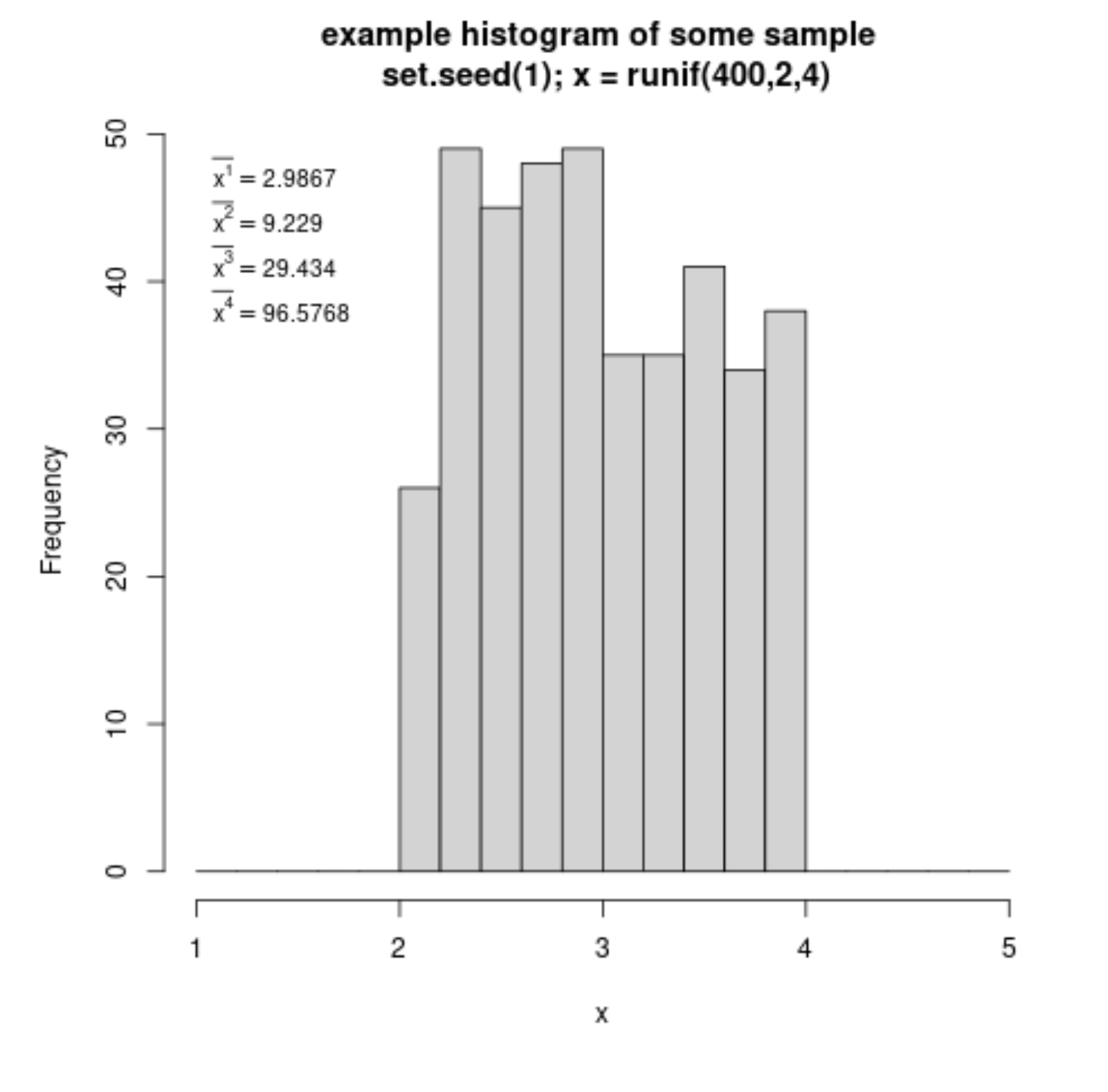
A sample could be something like set.seed(1); runif(400,2,4)

example of a sample

This sample is not exactly the same as a uniform distribution, and typically it will have different moments. That is, we can not find/fit a uniform distribution such that all moments of the fit and the moments of the sample are the same.

  • It is unlikely that some fit is possible such that all the moment of the fit and the sample are equal.

  • Instead, what the method of moments does is use only some specific moment(s) for the fit. The choice is arbitrary (depending on properties that are preferred) and makes it non-unique.

One of the ways, is to use the method of moments with the first two moments. We find/fit $a$ and $b$ such that $E[X] = \bar{X}$ and $E[X^2] = \bar{X^2}$. This happens when

$$m = \frac{a+b}{2} = \bar{X}$$ and $$d = b-a = \sqrt{ 12\left( \bar{X^2}-\bar{X}^2\right)}$$

So if we choose $a = 2.024179$ and $b = 3.949172$, then the moments of the fitted distribution are

$$ E[X] = 2.986675 \\ E[X^2] = 9.22903 \\ E[X^3] = 29.40869 \\ E[X^4] = 96.26954$$

and the first two of those moments are the same as the first two moments of the sample,

$$\bar{X} = 2.986675\\ \bar{X^2} = 9.22903\\ \bar{X^3} = 29.43404\\ \bar{X^4} = 96.5768$$

, but we could not make all moments the same.

$\endgroup$
0
2
$\begingroup$

Another simple example (cf. $\rm [I]$) where MoM estimators are not unique can be found in the case of parent population following noncentral chi-squared distribution with zero degrees of freedom and noncentrality parameter $\lambda.$ To see that, note

\begin{align}\mathbb E[X_i]&= \lambda,\\ \mathbb E[X_i^2]&=\lambda^2+4\lambda.\end{align}

But this post is not just for another example of non-uniqueness. For the sake of completion, it must be borne in mind that MoM estimators need not even exist. As $\rm[I]$ notes, the simplest examples are Cauchy, Uniform distribution on $(-\theta, \theta), ~\theta> 0;$ at least for the latter, higher order moments would be needed to construct an MoM estimator.

Suppose we have a single parameter $\theta$ and by MoM we equate the sample mean with $\mu(\theta), $ i.e. $\bar X=\mu(\theta). $ Then if $\mu^{-1}$ exists (and is continuous), we have our (consistent) MoM estimator $\mu^{-1}(\bar X) . $ The sufficient condition for this is $\mu^\prime(\theta) \ne 0.$

Consider now $X\sim \operatorname{Weibull}(\alpha); $ that is, $f(x;\alpha) =\alpha x^{\alpha-1}\exp(-x^\alpha), ~x> 0,\alpha > 0.$ Let $\theta:= \frac1\alpha +1.$ Now $\mu(\alpha) =\Gamma\left(\theta\right). $ But $\mu^{-1}$ doesn't exist: as $\Gamma(\theta) $ is differentiable and $\Gamma(1) =\Gamma(2) =1, $ by Rolle's theorem, there exists $\theta\in(1, 2) $ such that $\Gamma^\prime(\theta) =0.$ This in turn implies there exists $\alpha> 1$ such that $\mu^{-1}(\alpha) =0$ and this $\mu^{-1}$ doesn't exist invalidating the applicability of MoM. Things don't get pretty even if one takes into account higher moments: $\mu^\prime_k(\alpha) =\Gamma\left(\frac k\alpha +1\right) $ but the term in the parenthesis will vary over $(1, 2) $ making $\frac{\mathrm d\mu^\prime_k}{\mathrm d\alpha}=0.$

As reported by $\rm [II], $ simulation results showed that the minimum value of $\Gamma\left(\frac k\alpha +1\right) =0.8856;$ if observed $\mu^\prime_k(\alpha)<0.8856, $ the moment equation has no solution; if $\mu^\prime_k(\alpha)\in[0.8856, 1], $ then the moment equation would have two roots. And when $\mu^\prime_k(\alpha)> 1,$ then the moment equation provides a unique solution. (One can circumvent such intricacies by working with the transformed variable $\ln X$ which, by CLT, would face no problem in having an MoM estimator for very large samples).


References:

$\rm [I]$ Counterexamples in Probability and Statistics, Joseph P. Romano, Andrew F. Siegel, Wadsworth, $1986, $ examples $8.2, ~8.5,$ p. $177, ~179.$

$\rm [II]$ A First Course in Parametric Inference, B. K. Kale, Narosa Publishing, $1999, $ sec. $5.2, $ pp. $97-98.$

$\endgroup$
1
  • 1
    $\begingroup$ Thoughtful and crystal-clear and, +1! $\endgroup$
    – utobi
    Commented Jan 19 at 8:19

Your Answer

By clicking “Post Your Answer”, you agree to our terms of service and acknowledge you have read our privacy policy.

Not the answer you're looking for? Browse other questions tagged or ask your own question.