Sum of Products of Rademacher random variables

Question

Let $x_1 \ldots x_a,y_1 \ldots y_b$ be independent random variables taking values $+1$ or $-1$ with probability 0.5 each. Consider the sum $S = \sum_{i,j} x_i\times y_j$. I wish to upper bound the probability $P(|S| > t)$. The best bound I have right now is $2e^{-\frac{ct}{\max(a,b)}}$ where $c$ is a universal constant. This is achieved by lower bounding the probability $Pr(|x_1 + \dots + x_n|<\sqrt{t})$ and $Pr(|y_1 + \dots + y_n|<\sqrt{t})$ by application of simple Chernoff bounds. Can I hope to get something that is significantly better than this bound? For starters can I at least get $e^{-c\frac{t}{\sqrt{ab}}}$. If I can get sub-gaussian tails that would probably be the best but can we expect that (I don't think so but can't think of an argument)?

Answer 1

The algebraic relation

$$S = \sum_{i,j} x_i y_j = \sum_i x_i \sum_j y_j$$

exhibits $S$ as the product of two independent sums. Because $(x_i+1)/2$ and $(y_j+1)/2$ are independent Bernoulli$(1/2)$ variates, $X=\sum_{i=1}^a x_i$ is a Binomial$(a, 1/2)$ variable which has been doubled and shifted. Therefore its mean is $0$ and its variance is $a$. Similarly $Y=\sum_{j=1}^b y_j$ has a mean of $0$ and variance of $b$. Let's standardize them right now by defining

$$X_a = \frac{1}{\sqrt a} \sum_{i=1}^a x_i,$$

whence

$$S = \sqrt{ab} X_a X_b = \sqrt{ab}Z_{ab}.$$

To a high (and quantifiable) degree of accuracy, as $a$ grows large $X_a$ approaches the standard Normal distribution. Let us therefore approximate $S$ as $\sqrt{ab}$ times the product of two standard normals.

The next step is to notice that

$$Z_{ab} = X_aX_b = \frac{1}{2}\left(\left(\frac{X_a+X_b}{\sqrt 2}\right)^2 - \left(\frac{X_a-X_b}{\sqrt 2}\right)^2 \right) = \frac{1}{2}\left(U^2 - V^2\right).$$

is a multiple of the difference of the squares of independent standard Normal variables $U$ and $V$. The distribution of $Z_{ab}$ can be computed analytically (by inverting the characteristic function): its pdf is proportional to the Bessel function of order zero, $K_0(|z|)/\pi$. Because this function has exponential tails, we conclude immediately that for large $a$ and $b$ and fixed $t$, there is no better approximation to ${\Pr}_{a,b}(S \gt t)$ than given in the question.

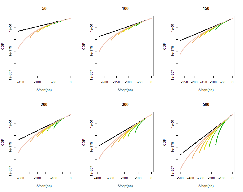
There remains some room for improvement when one (at least) of $a$ and $b$ is not large or at points in the tail of $S$ close to $\pm a b$. Direct calculations of the distribution of $S$ show a curved tapering off of the tail probabilities at points much larger than $\sqrt{ab}$, roughly beyond $\sqrt{ab\max(a,b)}$. These log-linear plots of the CDF of $S$ for various values of $a$ (given in the titles) and $b$ (ranging roughly over the same values as $a$, distinguished by color in each plot) show what's going on. For reference, the graph of the limiting $K_0$ distribution is shown in black. (Because $S$ is symmetric around $0$, $\Pr(S \gt t) = \Pr(-S \lt -t)$, so it suffices to look at the negative tail.)

As $b$ grows larger, the CDF grows closer to the reference line.

Characterizing and quantifying this curvature would require a finer analysis of the Normal approximation to Binomial variates.

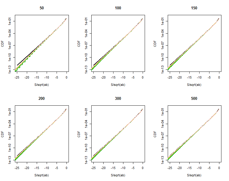
The quality of the Bessel function approximation becomes clearer in these magnified portions (of the upper right corner of each plot). We're already pretty far out into the tails. Although the logarithmic vertical scale can hide substantial differences, clearly by the time $a$ has reached $500$ the approximation is good for $|S| \lt a\sqrt{b}$.

---

R Code to Calculate the Distribution of $S$

The following will take a few seconds to execute. (It computes several million probabilities for 36 combinations of $a$ and $b$.) On slower machines, omit the larger one or two values of a and b and increase the lower plotting limit from $10^{-300}$ to around $10^{-160}$.

s <- function(a, b) {
  # Returns the distribution of S as a vector indexed by its support.
  products <- factor(as.vector(outer(seq(-a, a, by=2), seq(-b, b, by=2))))
  probs <- as.vector(outer(dbinom(0:a, a, 1/2), dbinom(0:b, b, 1/2)))
  tapply(probs, products, sum)
}

par(mfrow=c(2,3))
b.vec <- c(51, 101, 149, 201, 299, 501)
cols <- terrain.colors(length(b.vec)+1)
for (a in c(50, 100, 150, 200, 300, 500)) {
  plot(c(-sqrt(a*max(b.vec)),0), c(10^(-300), 1), type="n", log="y", 
       xlab="S/sqrt(ab)", ylab="CDF", main=paste(a))
  curve(besselK(abs(x), 0)/pi, lwd=2, add=TRUE)
  for (j in 1:length(b.vec)) {
    b <- b.vec[j]
    x <- s(a,b)
    n <- as.numeric(names(x))
    k <- n <= 0
    y <- cumsum(x[k])
    lines(n[k]/sqrt(a*b), y, col=cols[j], lwd=2)
  }
}

Answer 2

Comment: I edited the title in an attempt to reflect better what kind of r.v.'s are considered in the question. Anyone feel free to re-edit.

Motivation: I guess there is no need to settle for an upper bound, if we can derive the distribution of $|S_{ab}|$. (UPDATE: We can't -see Whuber's comments and answer).

Denote $Z_k = X_iY_j,\;\; k=1,...,ab$. It is easy to verify that $Z$'s have the same distribution as the $X$'s and the $Y$'s. The moment generating function is

$$M_Z(t) = E[e^{zt}]=\frac 12e^{-t}+\frac 12e^t = \cosh(t)$$

Moreover the $Z$'s are, to begin with, pair-wise independent: The variable $W = Z_1+Z_2$ (indices can be any of course), has support $\{-2,0,2\}$ with corresponding probabilities $\{1/4,1/2,1/4\}$. Its moment generating function is

$$M_{W}(t) = E[e^{(z_1+z_2)t}] = \frac 14e^{-2t}+\frac 12 +\frac 14e^{2t}=\\ =\frac 14(e^{-2t}+1)+ \frac 14(e^{2t}+1) = \frac 14 2e^{-t}\cosh(t)+\frac 14 2e^{t}\cosh(t)\\ =\cosh(t)\cdot \cosh(t) = M_{Z_1}(t)M_{Z_2}(t)$$

I will attempt to suspect that full independence holds, as follows (is it obvious to the wiser ones?): For this part, denote $Z_{ij}=X_iY_j$. Then by the chain rule $$P[Z_{ab},...,Z_{11}] = P[Z_{ab}\mid Z_{a,b-1},...,Z_{11}]\cdot ...\cdot P[Z_{13}\mid Z_{12},Z_{11}]\cdot P[Z_{12}\mid Z_{11}]\cdot P[Z_{11}]$$

By pair-wise independence we have $P[Z_{12}\mid Z_{11}] = P[Z_{12}]$.
Consider $P[Z_{13},Z_{12}\mid Z_{11}]$. $Z_{13}$ and $Z_{12}$ are independent conditional on $Z_{11}$ so we have $$P[Z_{13}\mid Z_{12},Z_{11}] = P[Z_{13}\mid Z_{11}] = P[Z_{13}]$$ the second equality by pair-wise independence. But this implies that

$$P[Z_{13}\mid Z_{12},Z_{11}]\cdot P[Z_{12}\mid Z_{11}]\cdot P[Z_{11}] = P[Z_{13},\,Z_{12},\,Z_{11}] = P[Z_{13}]\cdot P[Z_{12}]\cdot P[Z_{11}]$$

Etc (I think). ( UPDATE : I think wrong. Independence probably holds for any triplet, but not for the whole bunch. So what follows is just the derivation of the distribution of a simple random walk, and not a correct answer to the question - see Wolfies' and Whuber's answers).

If full independence does indeed hold, we have the task of deriving the distribution of a sum of i.i.d dichotomous r.v.'s $$S_{ab}=\sum_{k=1}^{ab}Z_k$$

which looks like a simple random walk, although without the clear interpretation of the latter as a sequence.

If $ab=even$ the support of $S$ will be the even integers in $[-ab,...,ab]$ including zero, while if $ab=odd$ the support of $S$ will be the odd integers in $[-ab,...,ab]$, without zero.

We treat the case of $ab=odd$.
Denote $m$ to be the number of $Z$'s taking the value $-1$. Then the support of $S$ can be written $S\in \{ab-2m;m\in \mathbb Z_+\cup\{0\};m\le ab\}$. For any given $m$, we obtain a unique value for $S$. Moreover, due to symmetric probabilities and independence (or just exchangeability?), all possible joint realizations of the $Z$-variables $\{Z_1=z_1,..., Z_{ab}=z_{ab}\}$ are equiprobable. So we count and we find that the probability mass function of $S$ is,

$$P(S=ab-2m)={ab \choose m}\cdot \frac 1{2^{ab}}, \qquad 0\le m\le ab$$

Defining $s\equiv ab-2m$, and odd number by construction, and the typical element of the support of $S$, we have

$$P(S=s)={ab \choose \frac{ab-s}{2}}\cdot \frac 1{2^{ab}}$$

Moving to $|S|$, since if $ab=odd$, the distribution of $S$ is symmetric around zero without allocating probability mass to zero, and so the distribution of $|S|$ is obtained by "folding" the density graph around the vertical axis, essentially doubling the probabilities for positive values,

$$P(|S|=|s|)={ab \choose \frac{ab-s}{2}}\cdot \frac 1{2^{ab-1}}$$

Then the distribution function is

$$P(|S|\le|s|)=\frac 1{2^{ab-1}}\sum_{1\le i\le s,\, i\,odd}{ab \choose \frac{ab-i}{2}}$$

Therefore, for any real $t$, $1\le t<ab$, we obtain the required probability $$P(|S|> t) = 1- P(|S|\le t) = 1-\frac 1{2^{ab-1}}\sum_{1\le i\le t,\, i\,odd}{ab \choose {\frac{ab-i}{2}}} $$

Note that the indication $i=odd$ guarantees that the sum will run only up to values included in the support of $|S|$ - for example, if we set $t=10.5$, still $i$ will run up to $9$, since it is constrained to be odd, on top of being an integer.

Answer 3

Not an answer, but a comment on Alecos’s interesting answer that is too long to fit into a comment box.

Let $(X_1, ..., X_a)$ be independent Rademacher random variables, and let $(Y_1, ..., Y_b)$ be independent Rademacher random variables. Alecos notes that:

$$S_{ab}=\sum_{k=1}^{ab}Z_k \qquad \text{where} \qquad Z_k = X_i Y_j$$

"… looks like a simple random walk”. If it were like a simple random walk, then the distribution of $S$ would be symmetric 'bell-shaped unimodal' around 0.

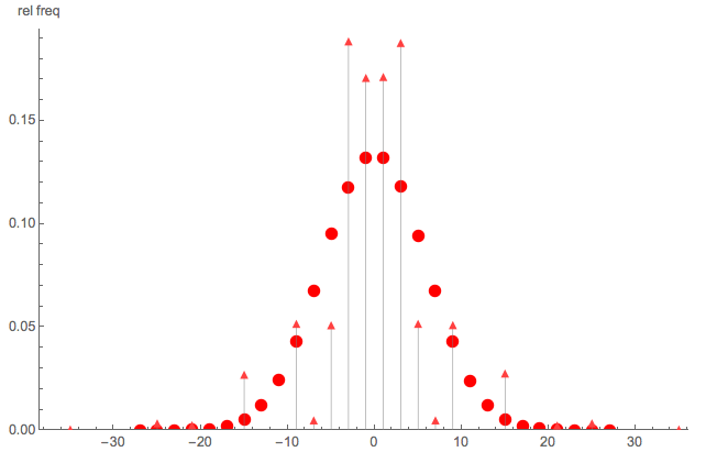
To illustrate that it is not a simple random walk, here is a quick Monte Carlo comparison of:

• triangle dots: Monte Carlo simulation of the pmf of $S$ given $a = 5$ and $b = 7$
• round dots: Monte Carlo simulation of a simple random walk with $n = 35$ steps

Clearly, $S$ is not a simple random walk; also note that S is not distributed on all the even (or odd) integers.

Monte Carlo

Here is the code (in Mathematica) used to generate a single iteration of the sum $S$, given $a$ and $b$:

 SumAB[a_, b_] :=  Outer[Times, RandomChoice[{-1, 1}, a], RandomChoice[{-1, 1}, b]] 
                         // Flatten // Total 

Then, 500,000 such paths, say when $a = 5$ and $b = 7$, can be generated with:

 data57 = Table[SumAB[5, 7], {500000}];

The domain of support for this combination of $a$ and $b$ is:

{-35, -25, -21, -15, -9, -7, -5, -3, -1, 1, 3, 5, 7, 9, 15, 21, 25, 35}